Multi-minimum Parameter Identification

This example is taken from [Vyasarayani2011]. In Section 3.1 there is a simple example of a single pendulum parameter identification that has many local minima.

For the following differential equations that describe a single pendulum acting under the influence of gravity, the goals is to identify the parameter p given noisy measurements of the angle, y1.

               --   --   --            --
               | y1' |   | y2           |
y' = f(y, t) = |     | = |              |
               | y2' |   | -p*sin(y1)   |
               --   --   --            --

import numpy as np
import sympy as sm
from scipy.integrate import odeint
import matplotlib.pyplot as plt
from opty import Problem

Specify the symbolic equations of motion.

p, t = sm.symbols('p, t')
y1, y2 = [f(t) for f in sm.symbols('y1, y2', cls=sm.Function)]
y = sm.Matrix([y1, y2])
f = sm.Matrix([y2, -p*sm.sin(y1)])
eom = y.diff(t) - f
sm.pprint(eom)

⎡            d           ⎤
⎢   -y₂(t) + ──(y₁(t))   ⎥
⎢            dt          ⎥
⎢                        ⎥
⎢               d        ⎥
⎢p⋅sin(y₁(t)) + ──(y₂(t))⎥
⎣               dt       ⎦

Generate some data by integrating the equations of motion.

duration = 50.0
num_nodes = 5000
interval = duration/(num_nodes - 1)
time = np.linspace(0.0, duration, num=num_nodes)

p_val = 10.0
y0 = [np.pi/6.0, 0.0]


def eval_f(y, t, p):
    return np.array([y[1], -p*np.sin(y[0])])


y_meas = odeint(eval_f, y0, time, args=(p_val,))
y1_meas = y_meas[:, 0]
y2_meas = y_meas[:, 1]

Add measurement noise.

y1_meas += np.random.normal(scale=0.05, size=y1_meas.shape)
y2_meas += np.random.normal(scale=0.1, size=y2_meas.shape)

Setup the optimization problem to minimize the error in the simulated angle and the measured angle. The midpoint integration method is preferable to the backward Euler method because no artificial damping is introduced.

def obj(free):
    """Minimize the error in the angle, y1."""
    return interval*np.sum((y1_meas - free[:num_nodes])**2)


def obj_grad(free):
    grad = np.zeros_like(free)
    grad[:num_nodes] = 2.0*interval*(free[:num_nodes] - y1_meas)
    return grad


prob = Problem(obj, obj_grad, eom, (y1, y2), num_nodes, interval,
               time_symbol=t, integration_method='midpoint')

num_states = len(y)

Give noisy measurements as the initial state guess and a random positive values as the parameter guess.

initial_guess = np.hstack((y1_meas, y2_meas, 100.0*np.random.random(1)))

Find the optimal solution.

solution, info = prob.solve(initial_guess)
p_sol = solution[-1]

Print the result.

known_msg = "Known value of p = {}".format(p_val)
guess_msg = "Initial guess for p = {}".format(initial_guess[-1])
identified_msg = "Identified value of p = {}".format(p_sol)
divider = '='*max(len(known_msg), len(identified_msg))

print(divider)
print(known_msg)
print(guess_msg)
print(identified_msg)
print(divider)

==========================================
Known value of p = 10.0
Initial guess for p = 45.42404253743789
Identified value of p = 10.001366458774221
==========================================

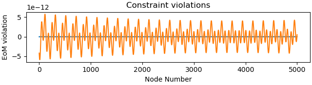
Plot constraint violations.

_ = prob.plot_constraint_violations(solution)

Simulate with the identified parameter.

y_sim = odeint(eval_f, y0, time, args=(p_sol,))
y1_sim = y_sim[:, 0]
y2_sim = y_sim[:, 1]

Plot results

fig_y1, axes_y1 = plt.subplots(3, 1, layout='constrained')

legend = ['measured', 'initial guess', 'direct collocation solution',
          'identified simulated']

axes_y1[0].plot(time, y1_meas, '.k',
                time, initial_guess[:num_nodes], '.b',
                time, solution[:num_nodes], '.r',
                time, y1_sim, 'g')
axes_y1[0].set_xlabel('Time [s]')
axes_y1[0].set_ylabel('y1 [rad]')
axes_y1[0].legend(legend)

axes_y1[1].set_title('Initial Guess Constraint Violations')
axes_y1[1].plot(prob.con(initial_guess)[:num_nodes - 1])
axes_y1[2].set_title('Solution Constraint Violations')
axes_y1[2].plot(prob.con(solution)[:num_nodes - 1])

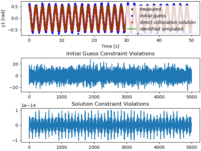
[<matplotlib.lines.Line2D object at 0x756106e5c440>]

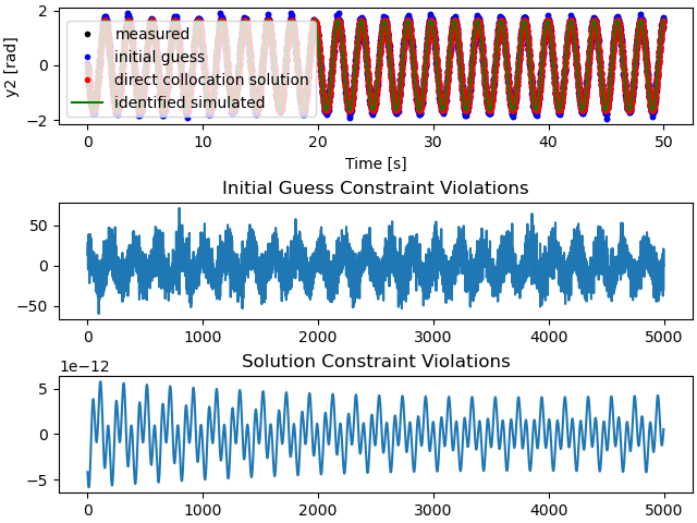
fig_y2, axes_y2 = plt.subplots(3, 1, layout='constrained')

axes_y2[0].plot(time, y2_meas, '.k',
                time, initial_guess[num_nodes:-1], '.b',
                time, solution[num_nodes:-1], '.r',
                time, y2_sim, 'g')
axes_y2[0].set_xlabel('Time [s]')
axes_y2[0].set_ylabel('y2 [rad]')
axes_y2[0].legend(legend)

axes_y2[1].set_title('Initial Guess Constraint Violations')
axes_y2[1].plot(prob.con(initial_guess)[num_nodes - 1:])
axes_y2[2].set_title('Solution Constraint Violations')
axes_y2[2].plot(prob.con(solution)[num_nodes - 1:])

plt.show()