Compare DAE vs. ODE Formulation

Objective

• To compare the results of the DAE and ODE formulations of the same problem. In one case one equation of motion is an algebraic equation (case 10.103), in the other case \(\dfrac{d}{dt}(\textrm{algebraic equation})\) is used.

Introduction

This is example 10.103 from [Betts2010]’s test problems. It has four differential equations and one algebraic equation. This example compares two solutions, the first uses the algebraic equation directly and the second uses the derivative of the algebraic equation, i.e. converts the DAEs to ODEs.

As expected, the DAE formulation gives a better result than the ODE formulation. The ODE formulation seems to run a bit faster.

States

• \(y_0,...,y_4\) : state variables

Specifieds

• \(u\) : control variable

import numpy as np
import sympy as sm
import sympy.physics.mechanics as me
from opty.direct_collocation import Problem
from opty.utils import create_objective_function

Information Common to Both Formulations

Define the time varying variables.

t = me.dynamicsymbols._t
y = me.dynamicsymbols('y0, y1, y2, y3, y4')
u = me.dynamicsymbols('u')

# Define the constant parameters.
g = 9.81

Set up the time intervals.

tf = 3.0
num_nodes = 751

t0, tf = 0.0, tf
interval_value = (tf - t0)/(num_nodes - 1)

Specify the objective function and form the gradient.

obj_func = sm.Integral(u**2, t)
sm.pprint(obj_func)
obj, obj_grad = create_objective_function(
    obj_func,
    y,
    (u,),
    tuple(),
    num_nodes,
    node_time_interval=interval_value,
    time_symbol=t,
)

⌠
⎮  2
⎮ u (t) dt
⌡

Specify the symbolic instance constraints.

instance_constraints = (
    y[0].func(t0) - 1,
    *[y[i].func(t0) - 0 for i in range(1, 5)],
    y[0].func(tf) - 0,
    y[2].func(tf) - 0,
)

Specify the bounds.

bounds = {
    y[0]: (-5, 5),
    y[1]: (-5, 5),
    y[2]: (-5, 5),
    y[3]: (-5, 5),
    y[4]: (-1, 15),
}

DAE Formulation

Define the differential algebraic equations of motion.

eom = sm.Matrix([
    -y[0].diff(t) + y[2],
    -y[1].diff(t) + y[3],
    -y[2].diff(t) - 2*y[4]*y[0] + u*y[1],
    -y[3].diff(t) - g - 2*y[4]*y[1] - u*y[0],
    y[2]**2 + y[3]**2 - 2*y[4] - g*y[1],
])
sm.pprint(eom)

⎡                      d                       ⎤
⎢              y₂(t) - ──(y₀(t))               ⎥
⎢                      dt                      ⎥
⎢                                              ⎥
⎢                      d                       ⎥
⎢              y₃(t) - ──(y₁(t))               ⎥
⎢                      dt                      ⎥
⎢                                              ⎥
⎢                                 d            ⎥
⎢    u(t)⋅y₁(t) - 2⋅y₀(t)⋅y₄(t) - ──(y₂(t))    ⎥
⎢                                 dt           ⎥
⎢                                              ⎥
⎢                              d               ⎥
⎢-u(t)⋅y₀(t) - 2⋅y₁(t)⋅y₄(t) - ──(y₃(t)) - 9.81⎥
⎢                              dt              ⎥
⎢                                              ⎥
⎢                   2        2                 ⎥
⎣   -9.81⋅y₁(t) + y₂ (t) + y₃ (t) - 2⋅y₄(t)    ⎦

Create the optimization problem and set any options.

prob = Problem(
    obj,
    obj_grad,
    eom,
    y,
    num_nodes,
    interval_value,
    instance_constraints=instance_constraints,
    bounds=bounds,
)

prob.add_option('nlp_scaling_method', 'gradient-based')

# Give rough estimates for the x and y trajectories.
initial_guess = np.zeros(prob.num_free)

# Find the optimal solution.
solution, info = prob.solve(initial_guess)
print(info['status_msg'])
if info['obj_val'] < 12.8738850:
    msg = 'opty with DAE gets a better result'
else:
    msg = 'opty with DAE gets a worse result'
print(f'Minimal objective value achieved: {info["obj_val"]:.4f},  ' +
      f'as per the book it is {12.8738850}, {msg} ')

obj_DAE = info["obj_val"]

b'Algorithm terminated successfully at a locally optimal point, satisfying the convergence tolerances (can be specified by options).'
Minimal objective value achieved: 12.0434,  as per the book it is 12.873885, opty with DAE gets a better result

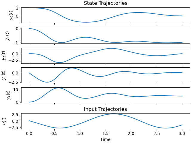
Plot the optimal state and input trajectories.

_ = prob.plot_trajectories(solution)

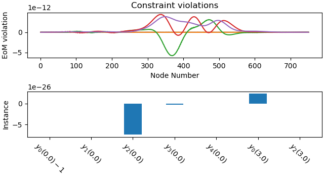
Plot the constraint violations.

_ = prob.plot_constraint_violations(solution)

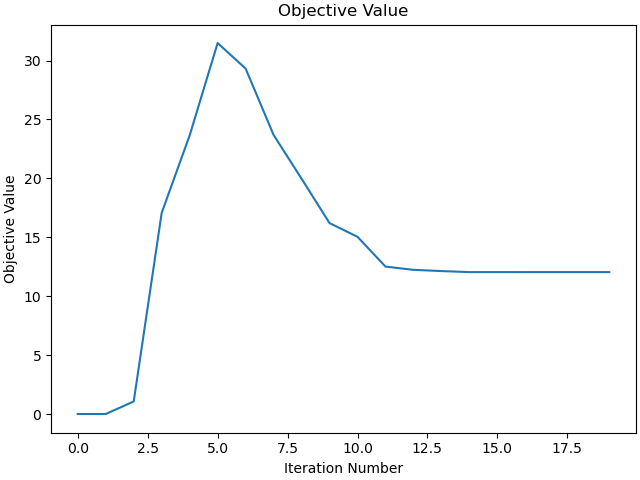
Plot the objective function as a function of optimizer iteration.

_ = prob.plot_objective_value()

ODE Formulation

Differentiate the algebraic equation with respect to time and add it to the equations of motion instead of the algebraic equation, as before.

eom = sm.Matrix([
    -y[0].diff(t) + y[2],
    -y[1].diff(t) + y[3],
    -y[2].diff(t) - 2*y[4]*y[0] + u*y[1],
    -y[3].diff(t) - g - 2*y[4]*y[1] - u*y[0],
    -y[4].diff(t) + y[2]*y[2].diff(t) + y[3]*y[3].diff(t) - g*y[1].diff(t)/2,
])
sm.pprint(eom)

⎡                               d                               ⎤
⎢                       y₂(t) - ──(y₀(t))                       ⎥
⎢                               dt                              ⎥
⎢                                                               ⎥
⎢                               d                               ⎥
⎢                       y₃(t) - ──(y₁(t))                       ⎥
⎢                               dt                              ⎥
⎢                                                               ⎥
⎢                                         d                     ⎥
⎢            u(t)⋅y₁(t) - 2⋅y₀(t)⋅y₄(t) - ──(y₂(t))             ⎥
⎢                                         dt                    ⎥
⎢                                                               ⎥
⎢                                      d                        ⎥
⎢        -u(t)⋅y₀(t) - 2⋅y₁(t)⋅y₄(t) - ──(y₃(t)) - 9.81         ⎥
⎢                                      dt                       ⎥
⎢                                                               ⎥
⎢      d                 d                 d           d        ⎥
⎢y₂(t)⋅──(y₂(t)) + y₃(t)⋅──(y₃(t)) - 4.905⋅──(y₁(t)) - ──(y₄(t))⎥
⎣      dt                dt                dt          dt       ⎦

Create the optimization problem and set any options.

prob = Problem(
    obj,
    obj_grad,
    eom,
    y,
    num_nodes,
    interval_value,
    instance_constraints=instance_constraints,
    bounds=bounds,
)

Find the optimal solution.

solution, info = prob.solve(initial_guess)
print(info['status_msg'])
if info['obj_val'] < 12.8738850:
    msg = 'opty with ODE gets a better result'
else:
    msg = 'opty with ODE gets a worse result'
print(f'Minimal objective value achieved: {info["obj_val"]:.4f},  ' +
      f'as per the book it is {12.8738850}, {msg} ')

obj_ODE = info["obj_val"]

b'Algorithm terminated successfully at a locally optimal point, satisfying the convergence tolerances (can be specified by options).'
Minimal objective value achieved: 12.5526,  as per the book it is 12.873885, opty with ODE gets a better result

Plot the optimal state and input trajectories.

_ = prob.plot_trajectories(solution)

Plot the constraint violations.

_ = prob.plot_constraint_violations(solution)

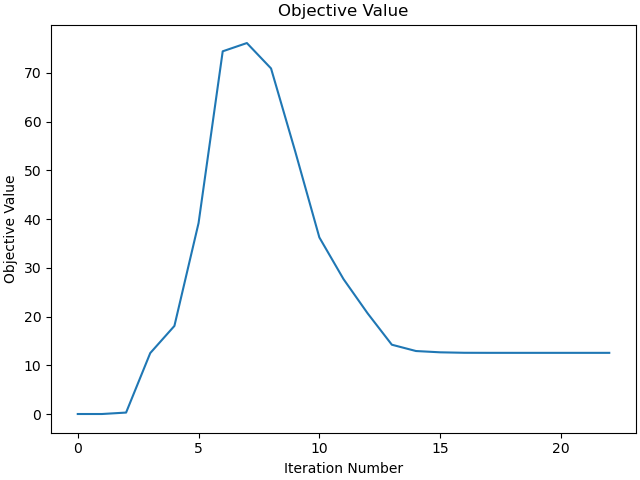
Plot the objective function as a function of optimizer iteration.

_ = prob.plot_objective_value()

Compare the results

if obj_DAE < obj_ODE:
    value = (obj_ODE - obj_DAE)/obj_ODE*100
    print(f'DAE formulation gives a better result by {value:.2f} %')
else:
    value = (obj_DAE - obj_ODE)/obj_DAE*100
    print(f'ODE formulation gives a better result by {value:.2f} %')

DAE formulation gives a better result by 4.06 %