Parameter Identification: Betts & Huffman 2003

This is the single parameter identification problem presented in section 7 of [Betts2003].

Objectives

• Show how to execute a parameter identification.

• Show how to handle time being explicit in the equations of motion using a known trajectory set to time.

import numpy as np
import sympy as sym
import matplotlib.pyplot as plt
from opty import Problem

duration = 1.0  # seconds
num_nodes = 100
interval = duration / (num_nodes - 1)

Define the variables.

mu, p, t = sym.symbols('mu, p, t')
y1, y2, T = sym.symbols('y1, y2, T', cls=sym.Function)

state_symbols = (y1(t), y2(t))
constant_symbols = (mu, p)

Define the symbolic equations of motion

Use a trick here because time was explicit in the eoms. Set T(t) to a function of time and then pass in time as a known trajectory in the problem.

eom = sym.Matrix([
    y1(t).diff(t) - y2(t),
    y2(t).diff(t) - mu**2 * y1(t) + (mu**2 + p**2) * sym.sin(p * T(t)),
])

Specify the known system parameters.

par_map = {mu: 60.0}

Generate data representing measurements of the system’s motion.

time = np.linspace(0.0, 1.0, num=num_nodes)
y1_m = np.sin(np.pi * time) + np.random.normal(scale=0.05, size=len(time))
y2_m = np.pi * np.cos(np.pi * time) + np.random.normal(scale=0.05,
                                                       size=len(time))

Specify the objective function and its gradient to minimize the sum of the squares of y1.

def obj(free):
    return interval * np.sum((y1_m - free[:num_nodes])**2)


def obj_grad(free):
    grad = np.zeros_like(free)
    grad[:num_nodes] = 2.0 * interval * (free[:num_nodes] - y1_m)
    return grad

Specify the symbolic instance constraints, i.e. initial and end conditions.

instance_constraints = (y1(0.0), y2(0.0) - np.pi)

Create an optimization problem.

prob = Problem(obj, obj_grad,
               eom, state_symbols,
               num_nodes, interval,
               known_parameter_map=par_map,
               known_trajectory_map={T(t): time},
               instance_constraints=instance_constraints,
               time_symbol=t,
               integration_method='midpoint')

Use a random positive initial guess.

initial_guess = np.random.randn(prob.num_free)

Find the optimal solution.

solution, info = prob.solve(initial_guess)
print(info['status_msg'])

b'Algorithm terminated successfully at a locally optimal point, satisfying the convergence tolerances (can be specified by options).'

Print results.

known_msg = "Known value of p = {}".format(np.pi)
identified_msg = "Identified value of p = {}".format(solution[-1])
divider = '=' * max(len(known_msg), len(identified_msg))

print(divider)
print(known_msg)
print(identified_msg)
print(divider)

==========================================
Known value of p = 3.141592653589793
Identified value of p = 3.1409353268742914
==========================================

Plot results.

fig_y1, axes_y1 = plt.subplots(3, 1, layout='constrained')

legend = ['measured', 'initial guess', 'direct collocation solution']

axes_y1[0].plot(time, y1_m, '.k',
                time, initial_guess[:num_nodes], '.b',
                time, solution[:num_nodes], '.r')
axes_y1[0].set_xlabel('Time [s]')
axes_y1[0].set_ylabel('y1')
axes_y1[0].legend(legend)

axes_y1[1].set_title('Initial Guess Constraint Violations')
axes_y1[1].plot(prob.con(initial_guess)[:num_nodes - 1])
axes_y1[2].set_title('Solution Constraint Violations')
axes_y1[2].plot(prob.con(solution)[:num_nodes - 1])

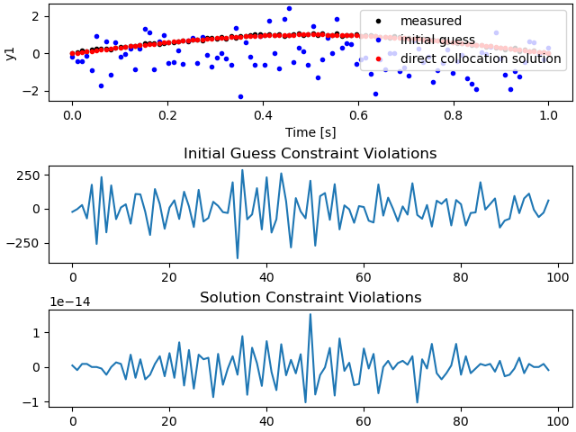
[<matplotlib.lines.Line2D object at 0x78c826df3a10>]

fig_y2, axes_y2 = plt.subplots(3, 1, layout='constrained')

axes_y2[0].plot(time, y2_m, '.k',
                time, initial_guess[num_nodes:-1], '.b',
                time, solution[num_nodes:-1], '.r')
axes_y2[0].set_xlabel('Time [s]')
axes_y2[0].set_ylabel('y2')
axes_y2[0].legend(legend)

axes_y2[1].set_title('Initial Guess Constraint Violations')
axes_y2[1].plot(prob.con(initial_guess)[num_nodes - 1:])
axes_y2[2].set_title('Solution Constraint Violations')
axes_y2[2].plot(prob.con(solution)[num_nodes - 1:])

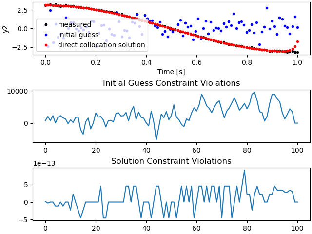
[<matplotlib.lines.Line2D object at 0x78c82733bcb0>]

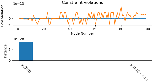
_ = prob.plot_constraint_violations(solution)

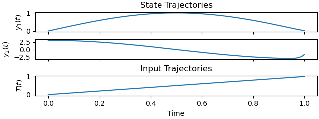
_ = prob.plot_trajectories(solution)

plt.show()