Fixed Duration Pendulum Swing Up

Objective

• Show the use of opty with likely the simplest example possible.

Introduction

Given a compound pendulum that is driven by a torque about its joint axis, swing the pendulum from hanging down to standing up in a fixed amount of time using minimal input torque with a bounded torque magnitude.

Notes

This example uses a fixed duration. There is an example which is mechanically identical to this one, but it uses a variable time interval, to get the pendulum up as fast as possible, given the torque limitations.

import numpy as np
import sympy as sm
from opty import Problem, create_objective_function
import matplotlib.pyplot as plt
import matplotlib.animation as animation

Start with defining the fixed duration and number of nodes.

duration = 10.0  # seconds
num_nodes = 501
interval_value = duration/(num_nodes - 1)

Specify the symbolic equations of motion.

I, m, g, d, t = sm.symbols('I, m, g, d, t')
theta, omega, T = sm.symbols('theta, omega, T', cls=sm.Function)

state_symbols = (theta(t), omega(t))
constant_symbols = (I, m, g, d)
specified_symbols = (T(t),)

eom = sm.Matrix([theta(t).diff() - omega(t),
                 I*omega(t).diff() + m*g*d*sm.sin(theta(t)) - T(t)])
sm.pprint(eom)

⎡                 d                 ⎤
⎢         -ω(t) + ──(θ(t))          ⎥
⎢                 dt                ⎥
⎢                                   ⎥
⎢  d                                ⎥
⎢I⋅──(ω(t)) + d⋅g⋅m⋅sin(θ(t)) - T(t)⎥
⎣  dt                               ⎦

Specify the known system parameters.

par_map = {
    I: 1.0,
    m: 1.0,
    g: 9.81,
    d: 1.0,
}

Specify the objective function and it’s gradient, in this case it calculates the area under the input torque curve over the simulation.

obj_func = sm.Integral(T(t)**2, t)
sm.pprint(obj_func)
obj, obj_grad = create_objective_function(obj_func, state_symbols,
                                          specified_symbols, tuple(),
                                          num_nodes,
                                          interval_value,
                                          time_symbol=t)

⌠
⎮  2
⎮ T (t) dt
⌡

Specify the symbolic instance constraints, i.e. initial and end conditions, where the pendulum starts a zero degrees (hanging down) and ends at 180 degrees (standing up).

target_angle = np.pi  # radians
instance_constraints = (
    theta(0.0),
    theta(duration) - target_angle,
    omega(0.0),
    omega(duration),
)

Limit the torque to a maximum magnitude.

bounds = {T(t): (-2.0, 2.0)}

Create an optimization problem.

prob = Problem(obj, obj_grad, eom, state_symbols, num_nodes, interval_value,
               known_parameter_map=par_map,
               instance_constraints=instance_constraints,
               bounds=bounds,
               time_symbol=t,
               backend='numpy')

# Use a random positive initial guess.
initial_guess = np.random.randn(prob.num_free)

Find the optimal solution.

solution, info = prob.solve(initial_guess)
print(info['status_msg'])
print(info['obj_val'])

b'Algorithm terminated successfully at a locally optimal point, satisfying the convergence tolerances (can be specified by options).'
15.641553623553241

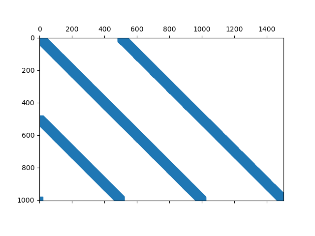
Plot the sparsity pattern of the Jacobian.

_ = prob.plot_jacobian_sparsity()

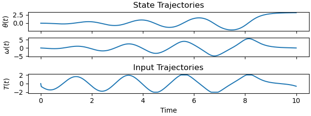
Plot the optimal state and input trajectories.

_ = prob.plot_trajectories(solution)

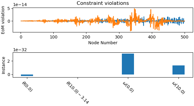
Plot the constraint violations.

_ = prob.plot_constraint_violations(solution)

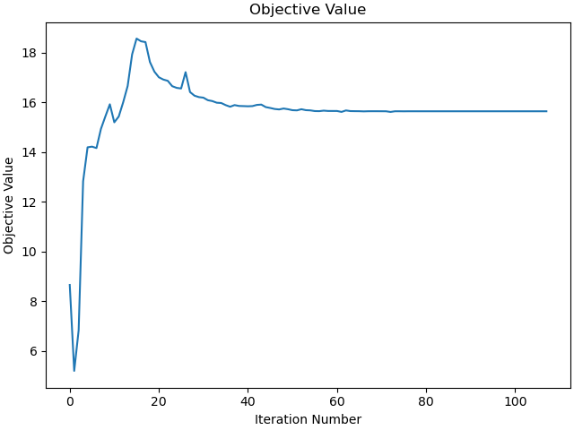
Plot the objective function as a function of optimizer iteration.

_ = prob.plot_objective_value()

Animate the pendulum swing up.

time = prob.time_vector()
angle = solution[:num_nodes]

fig = plt.figure()
ax = fig.add_subplot(111, aspect='equal', autoscale_on=False,
                     xlim=(-2, 2), ylim=(-2, 2))
ax.grid()

line, = ax.plot([], [], 'o-', lw=2)
time_template = 'time = {:0.1f}s'
time_text = ax.text(0.05, 0.9, '', transform=ax.transAxes)


def init():
    line.set_data([], [])
    time_text.set_text('')
    return line, time_text


def animate(i):
    x = [0, par_map[d]*np.sin(angle[i])]
    y = [0, -par_map[d]*np.cos(angle[i])]

    line.set_data(x, y)
    time_text.set_text(time_template.format(time[i]))
    return line, time_text


ani = animation.FuncAnimation(fig, animate, range(0, num_nodes, 4),
                              interval=int(interval_value*1000*4), blit=True,
                              init_func=init)

plt.show()

Once Loop Reflect