Delay Equation (Göllmann, Kern, and Maurer)

Objectives

• A simple example to show how to handle inequality constraints.

• Shows how instance constraints on one state variable may explicitly depend on an instance of another state variable at a different time.

Introduction

This is example 10.50 from [Betts2010].

States

• \(x_1, x_2, x_3. x_4. x_5, x_6\) : state variables

Controls

• \(u_1, u_2, u_3, u_4, u_5, u_6\) : control variables

import numpy as np
import sympy as sm
import sympy.physics.mechanics as me
import matplotlib.pyplot as plt
from opty.direct_collocation import Problem
from opty.utils import create_objective_function, MathJaxRepr

Equations of Motion

There are six differential equations:

\[\begin{split}\dot{x}_1 = & x_0 u_{-1} \\ \dot{x}_2 = & x_1 u_0 \\ \dot{x}_3 = & x_2 u_1 \\ \dot{x}_4 = & x_3 u_2 \\ \dot{x}_5 = & x_4 u_3 \\ \dot{x}_6 = & x_5 u_4\end{split}\]

and six algebraic inequality constraints:

\[\begin{split}0.3 \leq u_1 + x_1 \\ 0.3 \leq u_2 + x_2 \\ 0.3 \leq u_3 + x_3 \\ 0.3 \leq u_4 + x_4 \\ 0.3 \leq u_5 + x_5 \\ 0.3 \leq u_6 + x_6\end{split}\]

x1, x2, x3, x4, x5, x6 = me.dynamicsymbols('x1, x2, x3, x4, x5, x6')
u1, u2, u3, u4, u5, u6 = me.dynamicsymbols('u1, u2, u3, u4, u5, u6')
t = me.dynamicsymbols._t

x0 = 1.0
u_minus_1, u0 = 0.0, 0.0

eom = sm.Matrix([
    # equality constraints
    -x1.diff(t) + x0*u_minus_1,
    -x2.diff(t) + x1*u0,
    -x3.diff(t) + x2*u1,
    -x4.diff(t) + x3*u2,
    -x5.diff(t) + x4*u3,
    -x6.diff(t) + x5*u4,
    # inequality constraints
    u1 + x1,
    u2 + x2,
    u3 + x3,
    u4 + x4,
    u5 + x5,
    u6 + x6,
])
MathJaxRepr(eom)

$$\left[\begin{matrix}- \dot{x}_{1}\\- \dot{x}_{2}\\u_{1} x_{2} - \dot{x}_{3}\\u_{2} x_{3} - \dot{x}_{4}\\u_{3} x_{4} - \dot{x}_{5}\\u_{4} x_{5} - \dot{x}_{6}\\u_{1} + x_{1}\\u_{2} + x_{2}\\u_{3} + x_{3}\\u_{4} + x_{4}\\u_{5} + x_{5}\\u_{6} + x_{6}\end{matrix}\right]$$

Define and Solve the Optimization Problem

num_nodes = 501
t0, tf = 0.0, 1.0
interval_value = (tf - t0)/(num_nodes - 1)

state_symbols = (x1, x2, x3, x4, x5, x6)
unknown_input_trajectories = (u1, u2, u3, u4, u5, u6)

Specify the objective function and form the gradient.

objective = sm.Integral(
    x1**2 + x2**2 + x3**2 + x4**2 + x5**2 + x6**2 +
    u1**2 + u2**2 + u3**2 + u4**2 + u5**2 + u6**2, t)

obj, obj_grad = create_objective_function(
    objective,
    state_symbols,
    unknown_input_trajectories,
    tuple(),
    num_nodes,
    interval_value,
    time_symbol=t,
)

MathJaxRepr(objective)

$$\int \left(u_{1}^{2} + u_{2}^{2} + u_{3}^{2} + u_{4}^{2} + u_{5}^{2} + u_{6}^{2} + x_{1}^{2} + x_{2}^{2} + x_{3}^{2} + x_{4}^{2} + x_{5}^{2} + x_{6}^{2}\right)\, dt$$

Specify the instance constraints

instance_constraints = (
    x1.func(t0) - 1.0,
    x2.func(t0) - x1.func(tf),
    x3.func(t0) - x2.func(tf),
    x4.func(t0) - x3.func(tf),
    x5.func(t0) - x4.func(tf),
    x6.func(t0) - x5.func(tf),
    u1.func(t0) + x1.func(t0) - 0.5,
    u2.func(t0) + x2.func(t0) - 0.5,
    u3.func(t0) + x3.func(t0) - 0.5,
    u4.func(t0) + x4.func(t0) - 0.5,
    u5.func(t0) + x5.func(t0) - 0.5,
    u6.func(t0) + x6.func(t0) - 0.5,
)

Specify the bounds on the inequality constraints in the equations of motion. The key should match the corresponding index of the equation to apply the bounds to.

eom_bounds = {
    6: (0.3, np.inf),
    7: (0.3, np.inf),
    8: (0.3, np.inf),
    9: (0.3, np.inf),
    10: (0.3, np.inf),
    11: (0.3, np.inf),
}

Solve the Optimization Problem

prob = Problem(
    obj,
    obj_grad,
    eom,
    state_symbols,
    num_nodes,
    interval_value,
    instance_constraints=instance_constraints,
    time_symbol=t,
    backend='numpy',
    eom_bounds=eom_bounds,
)

prob.add_option('max_iter', 1000)

initial_guess = np.random.rand(prob.num_free)*0.1

solution, info = prob.solve(initial_guess)
initial_guess = solution
print(info['status_msg'])
print(f'Objective value achieved: {info["obj_val"]: .4f}, as per the book '
      f'it is {3.10812211}, so the error is: '
      f'{(info["obj_val"] - 3.10812211)/3.10812211*100: .3f} % ')
print('\n')

b'Algorithm terminated successfully at a locally optimal point, satisfying the convergence tolerances (can be specified by options).'
Objective value achieved:  3.1073, as per the book it is 3.10812211, so the error is: -0.027 %

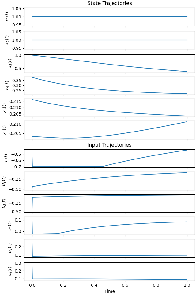
Plot the optimal state and input trajectories.

_ = prob.plot_trajectories(solution)

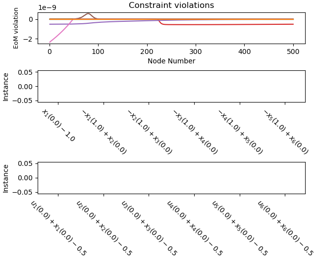
Plot the constraint violations. sphinx_gallery_thumbnail_number = 2

_ = prob.plot_constraint_violations(solution)

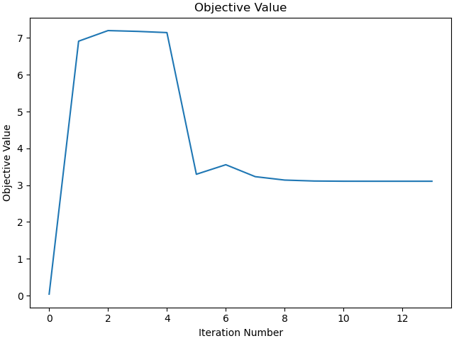
Plot the objective function.

_ = prob.plot_objective_value()

plt.show()