Hypersensitive Control

Objectives

• Show how opty works with a single differential equation.

• Shows how one can improve the accuracy by looking at the solution and changing parameters accordingly. (Here the solution is constant except near the beginning and near the end, so reducing the running time increases the accuracy, without having to resort to more nodes.)

• Uses a temporary directory to cache the compiled binary to avoid recompiling if the differential equations do not change.

Introduction

This is example 10.7 from [Betts2010]. As explained there, it was selected to be a very sensitive control problem.

States

• y : state variable

Specifieds

• u : control variable

import numpy as np
import sympy as sm
import sympy.physics.mechanics as me
from opty.direct_collocation import Problem
from opty.utils import create_objective_function

Equations of motion.

t = me.dynamicsymbols._t
y, u = me.dynamicsymbols('y u')

eom = sm.Matrix([-y.diff(t) - y**3 + u])
sm.pprint(eom)

⎡        3      d       ⎤
⎢u(t) - y (t) - ──(y(t))⎥
⎣               dt      ⎦

The optimization problem and its solution is packed into a function, so that you can easily call it with different parameters.

def solve_optimization(nodes, tf):
    t0, tf = 0.0, tf
    num_nodes = nodes
    interval_value = (tf - t0)/(num_nodes - 1)

    # Provide some reasonably realistic values for the constants.
    state_symbols = (y,)
    specified_symbols = (u,)

    # Specify the objective function and form the gradient.
    obj_func = sm.Integral(y**2 + u**2, t)
    sm.pprint(obj_func)
    obj, obj_grad = create_objective_function(
        obj_func, state_symbols, specified_symbols, tuple(), num_nodes,
        node_time_interval=interval_value, time_symbol=t)

    # Specify the symbolic instance constraints, as per the example.
    instance_constraints = (
        y.func(t0) - 1,
        y.func(tf) - 1.5,
    )

    # Create the optimization problem and set any options.
    prob = Problem(obj, obj_grad, eom, state_symbols, num_nodes,
                   interval_value, instance_constraints=instance_constraints,
                   time_symbol=t, tmp_dir='generated_code')

    prob.add_option('nlp_scaling_method', 'gradient-based')

    # Give some rough estimates for the trajectories.
    initial_guess = np.zeros(prob.num_free)

    # Find the optimal solution.
    solution, info = prob.solve(initial_guess)
    return solution, info, prob

As per the example tf = 10000.

tf = 10000
num_nodes = 501
solution, info, prob = solve_optimization(num_nodes, tf)
print(info['status_msg'])
print(f'Objective value achieved: {info["obj_val"]:.4f}, as per the book '
      f'it is {6.7241}, so the error is: '
      f'{(info["obj_val"] - 6.7241)/6.7241*100:.3f} % ')

⌠
⎮ ⎛ 2       2   ⎞
⎮ ⎝u (t) + y (t)⎠ dt
⌡
b'Algorithm terminated successfully at a locally optimal point, satisfying the convergence tolerances (can be specified by options).'
Objective value achieved: 282.5099, as per the book it is 6.7241, so the error is: 4101.453 %

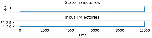
Plot the optimal state and input trajectories.

_ = prob.plot_trajectories(solution)

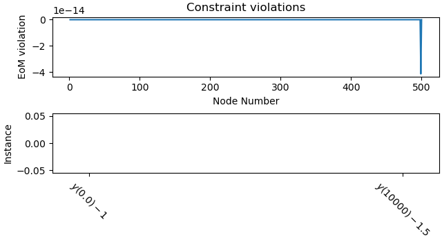
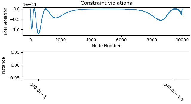
Plot the constraint violations.

_ = prob.plot_constraint_violations(solution)

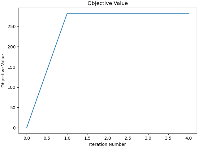
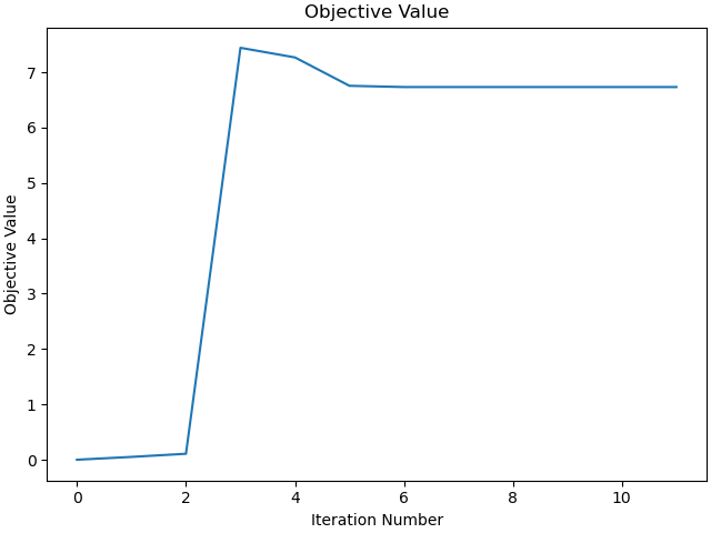
Plot the objective function as a function of optimizer iteration.

_ = prob.plot_objective_value()

With the value of tf = 10000 above, opty converged to a locally optimal point, but the objective value is far from the one given in the book. As per the plot of the solution y(t) it seems, that most of the time y(t) = 0, only at the very beginning and the very end it is different from 0. So, it may make sense to use a smaller tf. Also increasing num_nodes may help.

tf = 8.0
num_nodes = 10001
solution, info, prob = solve_optimization(num_nodes, tf)
print(info['status_msg'])
print(f'Objective value achieved: {info["obj_val"]:.4f}, as per the book '
      f'it is {6.7241}, so the error is: '
      f'{(info["obj_val"] - 6.7241)/6.7241*100:.3f} % ')

⌠
⎮ ⎛ 2       2   ⎞
⎮ ⎝u (t) + y (t)⎠ dt
⌡
b'Algorithm terminated successfully at a locally optimal point, satisfying the convergence tolerances (can be specified by options).'
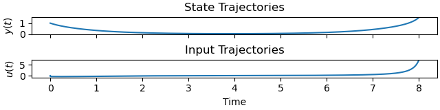
Objective value achieved: 6.7337, as per the book it is 6.7241, so the error is: 0.143 %

Plot the optimal state and input trajectories.

_ = prob.plot_trajectories(solution)

Plot the constraint violations.

_ = prob.plot_constraint_violations(solution)

Plot the objective function as a function of optimizer iteration.

_ = prob.plot_objective_value()