Path Constraints

Objectives

• Include additional path constraints in addition to the differential equations.

import numpy as np
import sympy as sm
import sympy.physics.mechanics as me
import matplotlib.pyplot as plt
from opty import Problem
from opty.utils import create_objective_function, MathJaxRepr

Introduction

Given a set of differential equations, any number of additional equations that are functions of the states can be appended to constrain the trajectories. These are typically called “path constraints”. Below the 6 ordinary differential equations of motion of a particle moving in space with an applied force are given. One algebraic path constraint is added to restrict the particle to being on the surface of a cylinder: Pythagoras’s theorem \(x^2 + y^2 = r^2\).

m, r = sm.symbols('m, r', real=True)
x, y, z = me.dynamicsymbols('x, y, z', real=True)
vx, vy, vz = me.dynamicsymbols('v_x, v_y, v_z', real=True)
Fx, Fy, Fz = me.dynamicsymbols('F_x, F_y, F_z', real=True)
t = me.dynamicsymbols._t

states = (x, y, z, vx, vy, vz)
specifieds = (Fx, Fy, Fz)

eom = sm.Matrix([
    x.diff() - vx,
    y.diff() - vy,
    z.diff() - vz,
    m*vx.diff() - Fx,
    m*vy.diff() - Fy,
    m*vz.diff() - Fz,
    x**2 + y**2 - r**2,
])
MathJaxRepr(eom)

$$\left[\begin{matrix}- v_{x} + \dot{x}\\- v_{y} + \dot{y}\\- v_{z} + \dot{z}\\m \dot{v}_{x} - F_{x}\\m \dot{v}_{y} - F_{y}\\m \dot{v}_{z} - F_{z}\\- r^{2} + x^{2} + y^{2}\end{matrix}\right]$$

Define the time and constant parameter numerical values.

num_nodes = 101
dt = 0.1
t0, tf = 0.0, dt*(num_nodes - 1)

par_map = {
    m: 1.0,
    r: 1.0,
}

Minimize the average force magnitude over time.

obj_func = sm.Integral(Fx**2 + Fy**2 + Fz**2, t)
obj, obj_grad = create_objective_function(
    obj_func, states, specifieds, tuple(), num_nodes,
    dt, time_symbol=t)
MathJaxRepr(obj_func)

$$\int \left(F_{x}^{2} + F_{y}^{2} + F_{z}^{2}\right)\, dt$$

Require that the particle make a half turn around the cylinder and rise a specified distance, \(4r\), being stationary at start and stop.

instance_constraints = (
    x.func(t0),
    y.func(t0) + r,
    z.func(t0),
    vx.func(t0),
    vy.func(t0),
    vz.func(t0),
    x.func(tf),
    y.func(tf) - r,
    z.func(tf) - 4*r,
    vx.func(tf),
    vy.func(tf),
    vz.func(tf),
)

Setup and solve the problem.

prob = Problem(
    obj,
    obj_grad,
    eom,
    states,
    num_nodes,
    dt,
    known_parameter_map=par_map,
    instance_constraints=instance_constraints,
    time_symbol=t,
    backend='numpy',
)

initial_guess = np.random.random(prob.num_free)
solution, info = prob.solve(initial_guess)

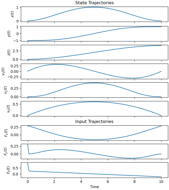
Plot the solution trajectories.

_ = prob.plot_trajectories(solution)

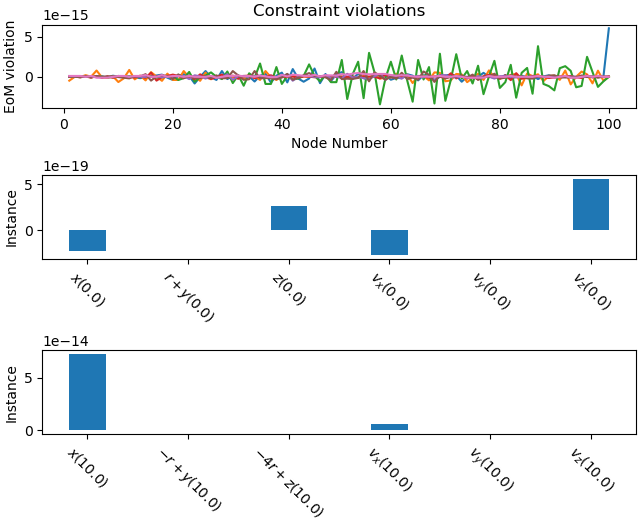
Plot the constraint violations.

_ = prob.plot_constraint_violations(solution)

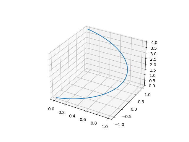
Show the path of the particle in 3D:

xs, _, _ = prob.parse_free(solution)
ax = plt.figure().add_subplot(projection='3d')
ax.plot(xs[0], xs[1], xs[2])

plt.show()