Hilly Race

Simulation of a particle subject to the force of gravity and air drag as it traverses an elevation profile with a specified numerical shape to reach the course finish line in minimal time.

Objectives

• Demonstrate generating a known trajectory via numerical functions.

• Show how interpolation can be used to generated a specified input.

import numpy as np
import sympy as sm
import sympy.physics.mechanics as me
import matplotlib.pyplot as plt
import matplotlib.animation as animation
from opty import Problem
from opty.utils import MathJaxRepr

Define the variables and equations of motion.

• \(m\): particle mass [kg]

• \(g\): acceleration due to gravity [m/s/s]

• \(h\): time step [s]

• \(s(t)\): distance traveled along elevation profile [m]

• \(v(t)\): longitudinal speed [m/s]

• \(x(t)\): horizontal coordinate [m]

• \(y(t)\): vertical coordinate [m]

• \(p(t)\): propulsion power [W]

• \(e(t)\): propulsion energy [J]

• \(\theta(x(t))\): slope angle [rad]

Note that the slope angle \(\theta\) is made a function of \(x(t)\) instead of simply \(t\). Numerical functions that generate \(\theta(x(t))\) and \(\frac{d\theta}{dx}\) will be supplied to incorporate this known trajectory into the equations of motion.

m, g, h = sm.symbols('m, g, h', real=True)
s, v, x, y, p, e = me.dynamicsymbols('s, v, x, y, p, e', real=True)
theta = sm.Function('theta')(x)

states = (x, y, s, v, e)

eom = sm.Matrix([
    x.diff() - v*sm.cos(theta),
    y.diff() - v*sm.sin(theta),
    s.diff() - v,
    m*v.diff() - p/v + m*g*sm.sin(theta) + v**2/3,
    e.diff() - p,
])
MathJaxRepr(eom)

$$\left[\begin{matrix}- v \cos{\left(\theta{\left(x \right)} \right)} + \dot{x}\\- v \sin{\left(\theta{\left(x \right)} \right)} + \dot{y}\\- v + \dot{s}\\g m \sin{\left(\theta{\left(x \right)} \right)} + m \dot{v} - \frac{p}{v} + \frac{v^{2}}{3}\\- p + \dot{e}\end{matrix}\right]$$

In the equations of motion, \(\theta(x(t))\) is present and will be specified as a known trajectory. When the Jacobian of the NLP constraint function is generated, \(\frac{d \theta}{dx}\) will also be required, so it will also be specified as a known trajectory.

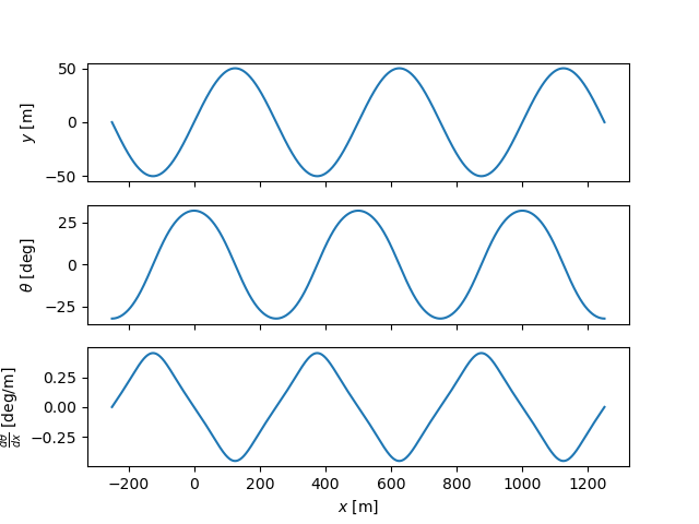
The elevation profile of a race course is often derived from measurements of a road surface. If a series of elevation values at specified linear distances are available, the slope is then also a function of the linear distances. The following code creates an elevation profile that simulates data collected from a road surface, albeit artificially smooth.

amp = 50.0
omega = 2*np.pi/500.0  # one period every 500 meters
x_meas = np.linspace(-250.0, 1250.0, num=3001)  # extend beyond expected range
y_meas = amp*np.sin(omega*x_meas)
theta_meas = np.arctan(amp*omega*np.cos(omega*x_meas))
dthetadx_meas = -amp*omega**2*np.sin(omega*x_meas)/(
    amp**2*omega**2*np.cos(omega*x_meas)**2 + 1)

fig, axes = plt.subplots(3, sharex=True)
axes[0].plot(x_meas, y_meas)
axes[0].set_ylabel(r'$y$ [m]')
axes[1].plot(x_meas, np.rad2deg(theta_meas))
axes[1].set_ylabel(r'$\theta$ [deg]')
axes[2].plot(x_meas, np.rad2deg(dthetadx_meas))
axes[2].set_ylabel(r'$\frac{d\theta}{dx}$ [deg/m]')
_ = axes[2].set_xlabel(r'$x$ [m]')

The following functions output the slope and its derivative with respect to \(x(t)\) at all values of \(x(t)\) using interpolation. The only input to these functions should be the optimization free vector and the output should be an array of values for \(\theta(t)\), one value for each node.

N = 201


def calc_theta(free):
    """
    Parameters
    ==========
    free : ndarray, shape(nN + qN + r + s, )

    Returns
    =======
    theta : ndarray, shape(N, )

    """
    x = free[0:N]
    return np.interp(x, x_meas, theta_meas)


def calc_dthetadx(free):
    """
    Parameters
    ==========
    free : ndarray, shape(nN + qN + r + s, )

    Returns
    =======
    dthetadx : ndarray, shape(N, )

    """
    x = free[0:N]
    return np.interp(x, x_meas, dthetadx_meas)

Minimize the time to reach the final distance traveled \(s(t_f)\) when starting from a standstill. The time step is the last value in free.

def obj(free):
    return free[-1]


def obj_grad(free):
    grad = np.zeros_like(free)
    grad[-1] = 1.0
    return grad

Start from a zero motion state and set the race duration to 1 kilometer.

t0, tf = 0*h, (N - 1)*h
sf = 1000.0  # meters
ef = 120000.0  # joules

instance_constraint = (
    x.func(t0),
    y.func(t0),
    s.func(t0),
    v.func(t0),
    e.func(t0),
    s.func(tf) - sf,
)

Limit the power and energy and make sure the speed and time step is positive.

bounds = {
    h: (0.0, 10.0),
    p: (0.0, 1000.0),
    v: (0.0, np.inf),
    e: (0.0, ef),
}

The slope angle \(\theta\) and its derivative \(\frac{d\theta}{dx}\) are set as a known trajectories and the functions calc_theta and calc_dthetadx functions are provided to generate the array of values dynamically during the optimization iterations.

prob = Problem(
    obj,
    obj_grad,
    eom,
    states,
    N,
    h,
    known_parameter_map={
        m: 100.0,  # kg
        g: 9.81,  # m/s/s
    },
    known_trajectory_map={
        theta.diff(x): calc_dthetadx,  # rad/m
        theta: calc_theta,  # rad
    },
    time_symbol=me.dynamicsymbols._t,
    instance_constraints=instance_constraint,
    bounds=bounds,
    integration_method='midpoint',
    backend='numpy',
)

Provide a linear initial guesses for each variable.

initial_guess = np.random.random(prob.num_free)
prob.fill_free(initial_guess, np.linspace(0.0, sf, num=N), x)
prob.fill_free(initial_guess, np.zeros(N), y)
prob.fill_free(initial_guess, np.linspace(0.0, sf, num=N), s)
prob.fill_free(initial_guess, 10.0*np.ones(N), v)
prob.fill_free(initial_guess, np.linspace(0.0, ef, num=N), e)
prob.fill_free(initial_guess, 500.0*np.ones(N), p)
prob.fill_free(initial_guess, 0.1, h)

_ = prob.plot_trajectories(initial_guess)

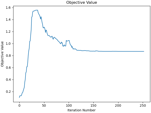
Solve the problem.

solution, info = prob.solve(initial_guess)

_ = prob.plot_objective_value()

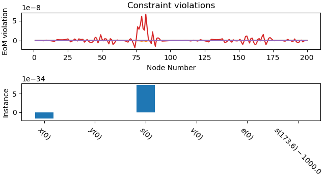
Plot the constraint violations.

_ = prob.plot_constraint_violations(solution)

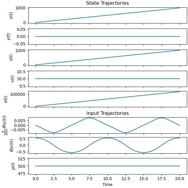
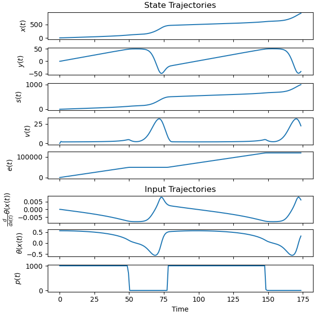
Plot the state and input solution trajectories.

_ = prob.plot_trajectories(solution)

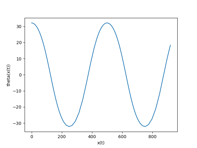
Plot the slope angle in degrees versus the horizontal distance.

x_vals = prob.extract_values(solution, x)
theta_vals = calc_theta(solution)
fig, ax = plt.subplots()
ax.plot(x_vals, np.rad2deg(theta_vals))
ax.set_xlabel(x)
_ = ax.set_ylabel(theta)

Animation of the particle traversing the profile: sphinx_gallery_thumbnail_number = 7

xs, rs, ps, dh = prob.parse_free(solution)

fig, ax = plt.subplots()
ax.plot(xs[0], xs[1])
dot, = ax.plot(xs[0, 0], xs[1, 0], marker='o', markersize=10)
ax.set_aspect('equal')
ax.set_ylabel(r'$y$ [m]')
ax.set_xlabel(r'$x$ [m]')


def animate(i):
    xi, yi = xs[0, i], xs[1, i]
    dot.set_data([xi], [yi])


ani = animation.FuncAnimation(fig, animate, range(0, N, 4))

plt.show()

Once Loop Reflect