Standing Balance Control Identification

Note

This example requires SciPy, symmeplot, yeadon, and PyDy in addition to opty and its required dependencies.

Objectives

• Demonstrate closed loop controller parameter identification on a realistic system.

• Demonstrate manual scaling for IPOPT.

Introduction

This example shows how to solve the human control parameter identification problem presented in [Park2004] using simulated noisy measurement data. The goal is to find a set of balance controller full-state feedback gains from data of perturbed standing balance. The dynamics model is a 2D planar two-body model representing a human standing on a antero-posteriorly moving platform. The dynamics model is developed in model_park_2004.py and the yeadon input parameters for the body segment properties are in JasonYeadonMeas.txt.

from opty import Problem
from opty.utils import sum_of_sines, MathJaxRepr
from scipy.integrate import odeint
from symmeplot.matplotlib import Scene3D
import matplotlib.pyplot as plt
import numpy as np
import sympy as sm

from model_park2004 import PlanarStandingHumanOnMovingPlatform

Equations of Motion

Generate the equations of motion and scale the control gains so that the values searched for with IPOPT are all close to 0.5 instead of the large gain values.

h = PlanarStandingHumanOnMovingPlatform(unscaled_gain=0.5)
h.derive()
eom = h.first_order_implicit()
MathJaxRepr(sm.simplify(eom))

$$\left[\begin{matrix}\omega_{a} - \dot{\theta}_{a}\\\omega_{h} - \dot{\theta}_{h}\\d_{L} g m_{L} \sin{\left(\theta_{a} \right)} + d_{L} m_{L} a \cos{\left(\theta_{a} \right)} + d_{T} g m_{T} \sin{\left(\theta_{a} + \theta_{h} \right)} + d_{T} l_{L} m_{T} \left(\omega_{a} + \omega_{h}\right)^{2} \sin{\left(\theta_{h} \right)} - d_{T} l_{L} m_{T} \omega_{a}^{2} \sin{\left(\theta_{h} \right)} + d_{T} m_{T} a \cos{\left(\theta_{a} + \theta_{h} \right)} + g l_{L} m_{T} \sin{\left(\theta_{a} \right)} - k_{00} s_{00} \theta_{a} - k_{01} s_{01} \theta_{h} - k_{02} s_{02} \omega_{a} - k_{03} s_{03} \omega_{h} + l_{L} m_{T} a \cos{\left(\theta_{a} \right)} - \left(I_{T} + d_{T} m_{T} \left(d_{T} + l_{L} \cos{\left(\theta_{h} \right)}\right)\right) \dot{\omega}_{h} - \left(I_{L} + I_{T} + d_{L}^{2} m_{L} + m_{T} \left(d_{T}^{2} + 2 d_{T} l_{L} \cos{\left(\theta_{h} \right)} + l_{L}^{2}\right)\right) \dot{\omega}_{a}\\d_{T} g m_{T} \sin{\left(\theta_{a} + \theta_{h} \right)} - d_{T} l_{L} m_{T} \omega_{a}^{2} \sin{\left(\theta_{h} \right)} + d_{T} m_{T} a \cos{\left(\theta_{a} + \theta_{h} \right)} - k_{10} s_{10} \theta_{a} - k_{11} s_{11} \theta_{h} - k_{12} s_{12} \omega_{a} - k_{13} s_{13} \omega_{h} - \left(I_{T} + d_{T}^{2} m_{T}\right) \dot{\omega}_{h} - \left(I_{T} + d_{T} m_{T} \left(d_{T} + l_{L} \cos{\left(\theta_{h} \right)}\right)\right) \dot{\omega}_{a}\end{matrix}\right]$$

Simulate Measurement Data

Define the time discretization.

num_nodes = 4000
duration = 20.0  # seconds
interval = duration/(num_nodes - 1)  # seconds
time = np.linspace(0.0, duration, num=num_nodes)

There are two types of noise that cause difficulties in parameter identification of controllers in closed loop systems. The first is process noise and it is added to the four states before entering the controller in a forward simulation. This represents the human’s inaccuracies in knowing its own plant model. This can be set to zero with process_noise = np.zeros((len(time), 4)) if desired.

process_noise = np.random.normal(scale=np.deg2rad(1.0), size=(len(time), 4))

The platform’s kinematics are specified as a sum of sinusoids to represent a pseudo-random perturbation of a wide bandwidth. The platform motion will drive the initial forward simulation but its motion would also be measured in the real experiment, so measurement noise is added later for use in the parameter identification.

nums = [7, 11, 16, 25, 38, 61, 103, 131, 151, 181, 313, 523]
freq = 2.0*np.pi*np.array(nums, dtype=float)/240.0
pos, vel, accel = sum_of_sines(0.02, freq, time)
accel_meas = accel + np.random.normal(scale=np.deg2rad(0.25), size=accel.shape)

Simulate the closed loop controlled motion of the human under the sinusoidal excitation and add Gaussian measurement noise (the second type of noise) to the resulting state trajectories to represent the motion measurements from a motion capture system, for example.

rhs, r, p = h.closed_loop_ode_func(time, process_noise, accel)
x0 = np.zeros(4)
x = odeint(rhs, x0, time, args=(r, p))
x_meas = x + np.random.normal(scale=np.deg2rad(0.25), size=x.shape)
x_meas_vec = x_meas.T.flatten()

Define Parameter Identification Problem

At this point there, all information for the parameter identification is available:

• plant model of the standing human with known geometry and inertial parameters

• feedback controller model with 8 unknown control gains the human used during the simulated balancing

• noisy measurements of the platform’s and human’s kinematics (position, velocity, acceleration)

To identify the eight gains, define an objective that minimizes the least square difference in the controlled plant’s motion and the measured motion:

\[J(\mathbf{p}_u) = \int_{t_0}^{t_f} \left[\mathbf{y}_\textrm{measured}(t) - \mathbf{y}_\textrm{simulated}(t) \right]^2 dt\]

def obj(free):
    """Minimize the error in all of the states."""
    return interval*np.sum((x_meas_vec - free[:4*num_nodes])**2)


def obj_grad(free):
    grad = np.zeros_like(free)
    grad[:4*num_nodes] = 2.0*interval*(free[:4*num_nodes] - x_meas_vec)
    return grad

The gains were scaled in the model definition to allow IPOPT to work with small magnitude values in the solution. The scaled gains should be between 0 and 1, so bound them. When working with real measurement data, more consideration may be needed for this scaling.

bounds = {}
for g in h.gain_symbols:
    bounds[g] = (0.0, 1.0)

Create the problem.

prob = Problem(
    obj,
    obj_grad,
    eom,
    h.states(),
    num_nodes,
    interval,
    known_parameter_map=h.closed_loop_par_map,
    known_trajectory_map={h.specified['platform_acceleration']: accel_meas},
    bounds=bounds,
    time_symbol=h.time,
    integration_method='midpoint',
)

Solve the Parameter Identification Problem

In such an experiment, the measurement data of the states can be used as an initial guess. Below are four possible initial guesses, all of which converge for this demo problem, with some taking IPOPT longer than others.

initial_guess = np.zeros(prob.num_free)
initial_guess = np.hstack((x_meas_vec, np.zeros(8)))
initial_guess = np.hstack((x_meas_vec, np.random.random(8)))
initial_guess = np.hstack((x_meas_vec,
                           (h.gain_scale_factors*h.numerical_gains).flatten()))

Find the optimal solution and compare to the values used to generate the data.

solution, info = prob.solve(initial_guess)
xs, rs, ps = prob.parse_free(solution)
print("Gain initial guess: {}".format(
    initial_guess[-8:]/h.gain_scale_factors.flatten()))
print("Known value of p = {}".format(
    h.numerical_gains.flatten()))
print("Identified value of p = {}".format(
    h.gain_scale_factors.flatten()*ps))

Gain initial guess: [950. 175. 185.  50.  45. 290.  60.  26.]
Known value of p = [950. 175. 185.  50.  45. 290.  60.  26.]
Identified value of p = [982.8102336  177.90033683 187.98424147  50.54625535  59.0471142
 292.56878627  59.9978948   25.44387377]

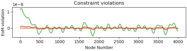
Plot the constraint violations.

_ = prob.plot_constraint_violations(solution)

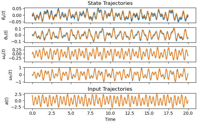
Show the difference in the measured state trajectories (blue) and the ones for the identified controller (orange).

axes = prob.plot_trajectories(initial_guess)
axes = prob.plot_trajectories(solution, axes=axes)

Below is an animation of the motion. sphinx_gallery_thumbnail_number = 3

def animate(fname='park2004.gif'):

    fig, ax = plt.subplots(subplot_kw={'projection': '3d'})

    scene = Scene3D(h.frames['inertial'], h.points['origin'], ax=ax)

    # create the platform
    scene.add_line([
        h.points['ankle'].locatenew('right', 0.3*h.frames['inertial'].x -
                                    0.02*h.frames['inertial'].y),
        h.points['ankle'].locatenew('left', -0.3*h.frames['inertial'].x -
                                    0.02*h.frames['inertial'].y),
    ], linewidth=6, color="tab:blue")

    shoulder = h.points['hip'].locatenew(
        'shoulder', 2*h.parameters['torso_com_length']*h.frames['torso'].y)

    # creates the stick person
    scene.add_line([
        h.points['ankle'].locatenew('left', -0.05*h.frames['inertial'].x),
        h.points['ankle'].locatenew('right', 0.15*h.frames['inertial'].x),
        h.points['ankle'],
        h.points['hip'],
        shoulder,
    ], linewidth=3, color="black")

    scene.add_point(h.points['hip'], color='tab:orange')
    scene.add_point(h.points['ankle'], color='tab:orange')
    scene.add_point(shoulder, color='tab:orange')

    # adds CoM and unit vectors for each body segment
    for body in h.rigid_bodies.values():
        scene.add_body(body)

    scene.lambdify_system(
        list(h.coordinates.values()) +
        list(h.speeds.values()) +
        list(h.specified.values()) +
        list(h.parameters.values())
    )

    y = np.vstack((
        xs,  # q, u shape(2n, N)  # solution
        np.atleast_2d(pos),  # x (1, N)
        np.zeros((4, len(time))),  # v, a, T_h, T_a
        np.repeat(np.atleast_2d(np.array(list(  # p, shape(r, N)
            h.open_loop_par_map.values()))).T, len(time), axis=1),
    ))

    scene.evaluate_system(*y[:, 0])

    scene.axes.set_proj_type("ortho")
    scene.axes.view_init(90, -90, 0)
    scene.plot()

    ani = scene.animate(lambda i: y[:, i], frames=range(0, len(time), 10))
    ani.save(fname)

    return ani


_ = animate()

Once Loop Reflect