Coulomb Friction with Linear Complimentarity Constraints

Objectives

• Demonstrate how linear complimentarity constraints and associated slack variables manage discontinuities in the dynamics.

Introduction

A block of mass \(m\) is being pushed with force \(F(t)\) along on a horizontal surface. Coulomb friction acts between the block and the surface. Find a minimal time solution to push the block 10 meters from being stationary and then back to the original stationary position.

The equations of motion of this system are:

\[\begin{split}\phantom{m}\dot{x} & = v \\ m\dot{v} & = F_f + F\end{split}\]

Coulomb friction force is a piecewise function defined as:

\[\begin{split}F_f = \begin{cases} \phantom{-}\mu_k m g & \textrm{if } v < 0 \\ \left[-\mu_s m g, \mu_s m g \right] & \textrm{if } v = 0 \\ -\mu_k m g & \textrm{if } v > 0 \\ \end{cases}\end{split}\]

This is a discontinuous nonlinear force. It is possible to convert discontinuous dynamics such as this into a set of linear complementarity constraints for the non-linear programming formulation that are continuous and differentiable. This requires more equations of motion and extra trajectories, but such a formulation is often better conditioned.

If \(F_f = F_{fp} - F_{fn}\) it breaks the friction into two positive components of force. Then the sum of the two positive valued friction components must always be less than or equal than the Coulomb magnitude (both could be zero):

\[\mu m g \geq F_{fp} + F_{fn}\]

The slack variable \(\psi\) is introduced and constrained to enforce it to be greater than \(|v|\), so \(\psi\) is always positive:

\[\begin{split}\psi \geq -v \\ \psi \geq v\end{split}\]

Using \(\psi\), the following two constraints then ensures that \(F_{fp}\) is zero if \(v > 0\) and \(F_{fn}\) is zero if \(v < 0\):

\[\begin{split}F_{fp} \psi = -F_{fp} v \\ F_{fn} \psi = F_{fn} v\end{split}\]

Again using \(\psi\), the following constraint ensures that \(\mu mg = F_{fn}\) if \(v > 0\) and \(\mu m g = F_{fp}\) and if \(v < 0\):

\[\mu m g \psi = (F_{fp} + F_{fn})\psi\]

[Posa2013] demonstrates that these constraints can be better conditioned if extra slack variables are introduced for each linear complimentarity constraint and the associated equality constraints are turned into inequality constraints. We have three linear complimentarity constraints, so three more slack variables are introduced and defined as:

\[\begin{split}\alpha & = \psi + v \geq 0 \\ \beta & = \psi - v \geq 0 \\ \gamma & = \mu mg - F_{fp} - F_{fn} \geq 0\end{split}\]

The equality constraints are then rewritten in terms of the new slack variables and as inequality constraints.

\[\begin{split}\alpha F_{fp} \leq 0 \textrm{ or } \epsilon\\ \beta F_{fn} \leq 0 \textrm{ or } \epsilon\\ \gamma \psi \leq 0 \textrm{ or } \epsilon\end{split}\]

\(\epsilon\) can be used to relax the inequality constraint and reduced during iterative solutions, but it is not needed for this simple problem.

import numpy as np
import sympy as sm
from opty import Problem
from opty.utils import MathJaxRepr
import matplotlib.pyplot as plt

Define all of the variables.

m, mu, g, t, h = sm.symbols('m, mu, g, t, h', real=True)
epsilon = sm.symbols('epsilon', real=True)

x, v, F = sm.symbols('x, v, F', cls=sm.Function)
psi, Ffp, Ffn = sm.symbols('psi, F_{fp}, F_{fn}', cls=sm.Function)
alpha, beta, gamma = sm.symbols('alpha, beta, gamma', cls=sm.Function)

Symbolic equations of motion.

eom = sm.Matrix([
    x(t).diff(t) - v(t),
    m*v(t).diff(t) - Ffp(t) + Ffn(t) - F(t),
    alpha(t) - psi(t) - v(t),
    beta(t) - psi(t) + v(t),
    gamma(t) - mu*m*g + Ffp(t) + Ffn(t),
    Ffp(t)*alpha(t) - epsilon,  # <= 0 [5]
    Ffn(t)*beta(t) - epsilon,  # <= 0 [6]
    gamma(t)*psi(t) - epsilon,  # <= 0 [7]
])
MathJaxRepr(eom)

$$\left[\begin{matrix}- v{\left(t \right)} + \frac{d}{d t} x{\left(t \right)}\\m \frac{d}{d t} v{\left(t \right)} - F{\left(t \right)} + F_{fn}{\left(t \right)} - F_{fp}{\left(t \right)}\\\alpha{\left(t \right)} - \psi{\left(t \right)} - v{\left(t \right)}\\\beta{\left(t \right)} - \psi{\left(t \right)} + v{\left(t \right)}\\- g m \mu + F_{fn}{\left(t \right)} + F_{fp}{\left(t \right)} + \gamma{\left(t \right)}\\- \epsilon + F_{fp}{\left(t \right)} \alpha{\left(t \right)}\\- \epsilon + F_{fn}{\left(t \right)} \beta{\left(t \right)}\\- \epsilon + \gamma{\left(t \right)} \psi{\left(t \right)}\end{matrix}\right]$$

Set the last three equations to be inequality constraints.

eom_bounds = {
    5: (-np.inf, 0.00),
    6: (-np.inf, 0.00),
    7: (-np.inf, 0.00),
}

Specify the objective function to minimize the time step and define its gradient.

def obj(free):
    """Return h (always the last element in the free variables)."""
    return free[-1]


def obj_grad(free):
    """Return the gradient of the objective."""
    grad = np.zeros_like(free)
    grad[-1] = 1.0
    return grad

Specify the symbolic instance constraints, i.e. initial, middle, and final conditions using node numbers 0 to N - 1.

N = 40

t0, tm, tf = 0*h, (N//2)*h, (N - 1)*h
instance_constraints = (
    x(t0) - 0.0,
    v(t0) - 0.0,
    x(tm) - 10.0,
    v(tm) - 0.0,
    x(tf) + 0.0,
    v(tf) - 0.0,
)

Bound all of the slack variables to be non-negative and provide reasonable bounds for the other variables.

bounds = {
    h: (0.0, 0.2),
    x(t): (0.0, 10.0),
    v(t): (-100.0, 100.0),
    F(t): (-400.0, 400.0),
    Ffp(t): (0.0, np.inf),
    Ffn(t): (0.0, np.inf),
    alpha(t): (0.0, np.inf),
    beta(t): (0.0, np.inf),
    gamma(t): (0.0, np.inf),
    psi(t): (0.0, np.inf),
}

Specify the known constant parameters.

par_map = {
    m: 1.0,
    mu: 0.6,
    g: 9.81,
    epsilon: 0.0,
}

Create the optimization problem.

prob = Problem(
    obj,
    obj_grad,
    eom,
    (x(t), v(t)),
    N,
    h,
    known_parameter_map=par_map,
    instance_constraints=instance_constraints,
    time_symbol=t,
    bounds=bounds,
    eom_bounds=eom_bounds,
    backend='numpy',
)

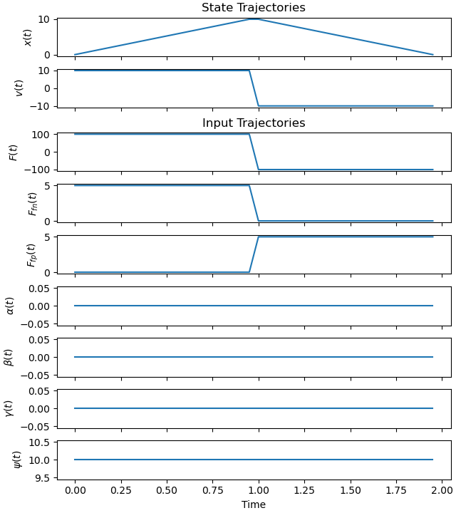
Provide an initial guess that has similarity to the expected solution.

half = N//2
initial_guess = np.zeros(prob.num_free)

initial_guess[0*N:1*N - half] = np.linspace(0.0, 10.0, num=half)  # x
initial_guess[1*N - half:1*N] = np.linspace(10.0, 0.0, num=half)  # x

initial_guess[1*N:2*N - half] = 10.0  # v
initial_guess[2*N - half:2*N] = -10.0  # v

initial_guess[2*N:3*N - half] = 100.0  # F
initial_guess[3*N - half:3*N] = -100.0  # F

initial_guess[3*N:4*N - half] = 5.0  # Ffn
initial_guess[4*N - half:4*N] = 0.0  # Ffn

initial_guess[4*N:5*N - half] = 0.0  # Ffp
initial_guess[5*N - half:5*N] = 5.0  # Ffp

initial_guess[8*N:9*N - half] = 10.0  # psi
initial_guess[9*N - half:9*N] = 10.0  # psi

initial_guess[-1] = 0.05

Plot the initial guess.

_ = prob.plot_trajectories(initial_guess)

Find the optimal solution.

solution, info = prob.solve(initial_guess)
print(info['status_msg'])
print('Minimal time step: {:1.3f} s'.format(info['obj_val']))
print('Time to slide the block: {:1.2f} s'.format(solution[-1]*(N - 1)))

b'Algorithm terminated successfully at a locally optimal point, satisfying the convergence tolerances (can be specified by options).'
Minimal time step: 0.017 s
Time to slide the block: 0.65 s

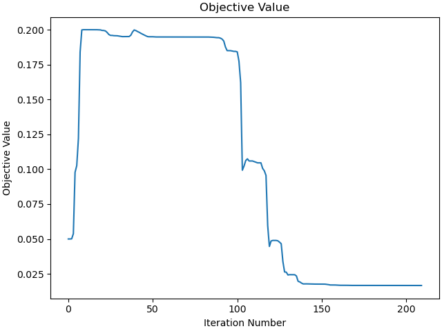
Plot the objective function as a function of optimizer iteration.

_ = prob.plot_objective_value()

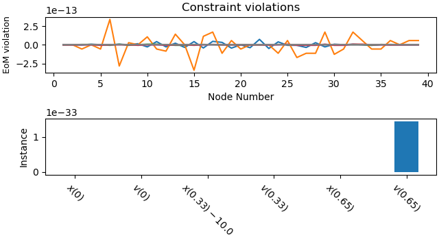
Plot the constraint violations.

_ = prob.plot_constraint_violations(solution)

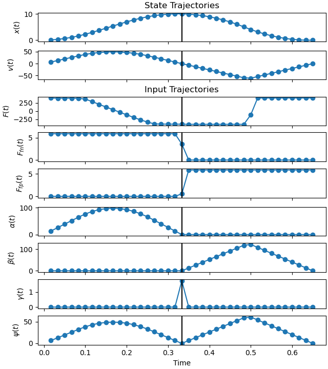
Plot the optimal state and input trajectories (skips the first node because it is not dynamically constrained due to backward Euler method).

axes = prob.plot_trajectories(solution)
for ax in axes:
    lines = ax.get_lines()
    for line in lines:
        line.set_marker('o')
        x, y = line.get_data()
        x[0], y[0] = np.nan, np.nan
        line.set_data(x, y)
    ax.relim()
    ax.autoscale_view(tight=True)
    ax.axvline(N//2*solution[-1], color='black')

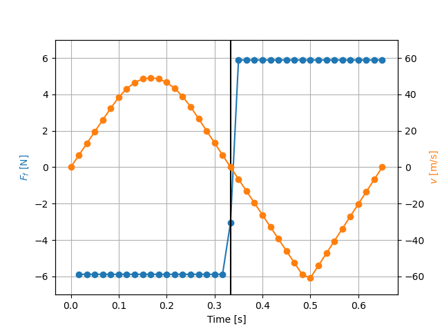
Plot the friction force (skips the first node because it is not dynamically constrained due to backward Euler method).

t_vals = prob.time_vector(solution)
Ffp_vals = prob.extract_values(solution, Ffp(t))
Ffn_vals = prob.extract_values(solution, Ffn(t))
v_vals = prob.extract_values(solution, v(t))

fig, ax = plt.subplots()
ax.plot(t_vals[1:], Ffp_vals[1:] - Ffn_vals[1:], marker='o')
ax.axvline(N//2*solution[-1], color='black')
ax.set_ylim((-7.0, 7.0))
ax.set_ylabel(r'$F_f$ [N]', color='C0')
ax.set_xlabel('Time [s]')
ax_r = ax.twinx()
ax_r.plot(t_vals, v_vals, marker='o', color='C1')
ax_r.set_ylabel(r'$v$ [m/s]', color='C1')
ax_r.set_ylim((-70.0, 70.0))
ax.grid()

plt.show()