Park a Car in a Garage

Objectives

• Shows how use inequalities in the equations of motion.

• Shows how a differentiable minimum function in connection with an unknown input trajectory may be used to ‘know’ the minimum at all times.

Introduction

A conventional car is modeled: The rear axle is driven, the front axle does the steering. No speed possible perpendicular to the wheels. The car must enter the garage without colliding with the walls. opty is ‘free’ to to ‘decide’ whether the car backs into the garage or goes in forward.

Detailed Description on how the Objectives are Achieved

• the garage is modeled as a differentiable trough.

• number of points evenly spread on the body of the car are considered.

• the y-coordinates of these points must be above the trough at all times.

• as it is not clear a priori whether the car will drive straight into the garage or back in, the variable pmin is introduced, which is the lower end of the car. To ackomplish this, a differentiable version of the minimum function is used.

states

• \(x, y\): coordinates of the front of the car

• \(u_x, u_y\): velocities of the front of the car

• \(q_0, q_f\): orientation of the car and the steering angle of the front axle

• \(u_0, u_f\): angular velocities of the car and the front axle

controls

• \(T_f\): steering torque on the front axle

• \(F_b\): driving force on the rear axle

• \(p_{min}\): the lowest point of the car

parameters

• \(l\): length of the car

• \(m_0, m_b, m_f\): mass of the car, the rear and the front axle

• \(i_{ZZ_0}, i_{ZZ_b}, i_{ZZ_f}\): moments of inertia of the car, the rear and the front axle

• \(reibung\): friction coefficient

• \(x_1, x_2, y_{12}\): the shape of the garage

import os
import sympy.physics.mechanics as me
import numpy as np
import sympy as sm
from scipy.interpolate import CubicSpline

from opty.direct_collocation import Problem
from opty.utils import create_objective_function
import matplotlib.pyplot as plt
from matplotlib.animation import FuncAnimation

Kane’s Equations of Motion

N, A0, Ab, Af = sm.symbols('N A0 Ab Af', cls=me.ReferenceFrame)
t = me.dynamicsymbols._t
O, Pb, Dmc, Pf = sm.symbols('O Pb Dmc Pf', cls=me.Point)
O.set_vel(N, 0)

q0, qf = me.dynamicsymbols('q_0 q_f')
u0, uf = me.dynamicsymbols('u_0 u_f')
x, y = me.dynamicsymbols('x y')
ux, uy = me.dynamicsymbols('u_x u_y')
Tf, Fb = me.dynamicsymbols('T_f F_b')
reibung = sm.symbols('reibung')

l, m0, mb, mf, iZZ0, iZZb, iZZf = sm.symbols('l m0 mb mf iZZ0, iZZb, iZZf')

A0.orient_axis(N, q0, N.z)
A0.set_ang_vel(N, u0 * N.z)

Ab.orient_axis(A0, 0, N.z)

Af.orient_axis(A0, qf, N.z)
rot = Af.ang_vel_in(N)
Af.set_ang_vel(N, uf * N.z)
rot1 = Af.ang_vel_in(N)

Pf.set_pos(O, x * N.x + y * N.y)
Pf.set_vel(N, ux * N.x + uy * N.y)

Pb.set_pos(Pf, -l * A0.y)
Pb.v2pt_theory(Pf, N, A0)

Dmc.set_pos(Pf, -l/2 * A0.y)
Dmc.v2pt_theory(Pf, N, A0)
prevent_print = 1.

No speed perpendicular to the wheels.

vel1 = me.dot(Pb.vel(N), Ab.x) - 0
vel2 = me.dot(Pf.vel(N), Af.x) - 0

I0 = me.inertia(A0, 0, 0, iZZ0)
body0 = me.RigidBody('body0', Dmc, A0, m0, (I0, Dmc))
Ib = me.inertia(Ab, 0, 0, iZZb)
bodyb = me.RigidBody('bodyb', Pb, Ab, mb, (Ib, Pb))
If = me.inertia(Af, 0, 0, iZZf)
bodyf = me.RigidBody('bodyf', Pf, Af, mf, (If, Pf))
BODY = [body0, bodyb, bodyf]

FL = [(Pb, Fb * Ab.y), (Af, Tf * N.z), (Dmc, -reibung * Dmc.vel(N))]

kd = sm.Matrix([ux - x.diff(t), uy - y.diff(t), u0 - q0.diff(t),
                me.dot(rot1 - rot, N.z)])
speed_constr = sm.Matrix([vel1, vel2])

q_ind = [x, y, q0, qf]
u_ind = [u0, uf]
u_dep = [ux, uy]

KM = me.KanesMethod(
                    N, q_ind=q_ind, u_ind=u_ind,
                    kd_eqs=kd,
                    u_dependent=u_dep,
                    velocity_constraints=speed_constr,
                    )
(fr, frstar) = KM.kanes_equations(BODY, FL)

eom = kd.col_join(fr + frstar)
eom = eom.col_join(speed_constr)
print(f'the dynamic part of the equations of motion has {eom.shape} shape')

the dynamic part of the equations of motion has (8, 1) shape

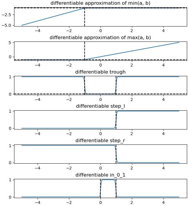
Define the various differentiable approximations.

def min_diff(a, b, gr):
    # differentiabl approximation of min(a, b)
    # the higher gr the closer the approximation
    return -1/gr * sm.log(sm.exp(-gr * a) + sm.exp(-gr * b))


def max_diff(a, b, gr):
    # differentiabl approximation of max(a, b)
    # the higher gr the closer the approximation
    return 1/gr * sm.log(sm.exp(gr * a) + sm.exp(gr * b))


def trough(x, a, b, gr):
    # approx zero for x in [a, b]
    # approx one otherwise
    # the higher gr the closer the approximation
    return 1/(1 + sm.exp(gr*(x - a))) + 1/(1 + sm.exp(-gr*(x - b)))


def step_l_diff(a, b, gr):
    # approx zero for a < b, approx one otherwise
    return 1/(1 + sm.exp(-gr*(a - b)))


def step_r_diff(a, b, gr):
    # approx zero for a > b, approx one otherwise
    return 1/(1 + sm.exp(gr*(a - b)))


def in_0_1(x):
    wert = (step_l_diff(x, 0, 50) * step_r_diff(x, 1, 50)
            * (1-trough(x, 0, 1, 50)))
    return wert

Add the equations of motion which constrain the car. \(\delta_p\) is the distance of the points on the car to the trough. number gives the number of points on the body of the car which are considered.

number = 4

x1, x2, y12 = sm.symbols('x1 x2 y12')
pmin = me.dynamicsymbols('pmin')

park1y = Pf.pos_from(O).dot(N.y)
park2y = Pb.pos_from(O).dot(N.y)
park1x = Pf.pos_from(O).dot(N.x)
park2x = Pb.pos_from(O).dot(N.x)

delta_x = [park1x + (park2x - park1x)*i/(number - 1) for i in range(number)]
delta_y = [park1y + (park2y - park1y)*i/(number - 1) for i in range(number)]

delta_p = [delta_y[i] - trough(delta_x[i], x1, x2, 50)*y12
           for i in range(number)]

eom_add = sm.Matrix([
    *[delta_p[i] for i in range(number)],
    -pmin + min_diff(park1y, park2y, 50),
])
eom = eom.col_join(eom_add)
print((f'the eoms are too large to be printed here. The shape is {eom.shape}'
       f' and they contain {sm.count_ops(eom)} operations.'))

the eoms are too large to be printed here. The shape is (13, 1) and they contain 567 operations.

Check what the differentiable approximations of max(a, b), min(a, b), trough(a, b) and x \(\in\) [0, 1] look like.

a, b, c, gr = sm.symbols('a b c gr')
min_diff_lam = sm.lambdify((x, b, gr), min_diff(x, b, gr))
max_diff_lam = sm.lambdify((x, b, gr), max_diff(x, b, gr))
trough_lam = sm.lambdify((x, a, b, gr), trough(x, a, b, gr))
step_l_diff_lam = sm.lambdify((a, b, gr), step_l_diff(a, b, gr))
step_r_diff_lam = sm.lambdify((a, b, gr), step_r_diff(a, b, gr))
in_0_1_lam = sm.lambdify(x, in_0_1(x))

a = -1.0
b = 1.0
c = 6.0
gr = 50
XX = np.linspace(-5.0, 5.0, 200)
fig, ax = plt.subplots(6, 1, figsize=(6.4, 7), constrained_layout=True)
ax[0].plot(XX, min_diff_lam(XX, a, gr))
ax[0].axhline(a, color='k', linestyle='--')
ax[0].axvline(a, color='k', linestyle='--')
ax[0].set_title('differentiable approximation of min(a, b)')


ax[1].plot(XX, max_diff_lam(XX, a, gr))
ax[1].axhline(a, color='k', linestyle='--')
ax[1].axvline(a, color='k', linestyle='--')
ax[1].set_title('differentiable approximation of max(a, b)')


ax[2].plot(XX, trough_lam(XX, a, b, gr))
ax[2].axvline(a, color='k', linestyle='--')
ax[2].axvline(b, color='k', linestyle='--')
ax[2].axhline(0, color='k', linestyle='--')
ax[2].set_title('differentiable trough')

ax[3].plot(XX, step_l_diff_lam(XX, b, gr))
ax[3].axvline(b, color='k', linestyle='--')
ax[3].set_title('differentiable step_l')

ax[4].plot(XX, step_r_diff_lam(XX, b, gr))
ax[4].axvline(b, color='k', linestyle='--')
ax[4].set_title('differentiable step_r')

ax[5].plot(XX, in_0_1_lam(XX))
ax[5].axvline(0, color='k', linestyle='--')
ax[5].axvline(1, color='k', linestyle='--')
ax[5].set_title('differentiable in_0_1')
prevent_print = 1.

Set the Optimization Problem and Solve It

state_symbols = (x, y, q0, qf, ux, uy, u0, uf)
constant_symbols = (l, m0, mb, mf, iZZ0, iZZb, iZZf, reibung)
specified_symbols = (Fb, Tf, pmin)
unknown_symbols = ()

num_nodes = 301
t0, tf = 0.0, 5.0
interval_value = (tf - t0) / (num_nodes - 1)

Specify the known system parameters.

par_map = {}
par_map[m0] = 1.0
par_map[mb] = 0.5
par_map[mf] = 0.5
par_map[iZZ0] = 1.
par_map[iZZb] = 0.5
par_map[iZZf] = 0.5
par_map[l] = 3.0
par_map[reibung] = 0.5
par_map[x1] = -0.75
par_map[x2] = 0.75
par_map[y12] = 5.0

Specify the objective function, the constraints and the bounds.

objective = sm.Integral(Fb**2 + Tf**2, t)
obj, obj_grad = create_objective_function(
    objective,
    state_symbols,
    specified_symbols,
    tuple(),
    num_nodes,
    interval_value,
    time_symbol=t,
)

instance_constraints = (
    x.func(t0) - 7.5,
    y.func(t0) - 5.5,
    q0.func(t0) - np.pi/2.0,
    qf.func(t0) - 0.5,
    ux.func(t0) - 0.0,
    uy.func(t0) - 0.0,
    u0.func(t0) - 0.0,
    uf.func(t0) - 0.0,
    pmin.func(tf) - 0.5,
    x.func(tf) - 0.0,
    ux.func(tf) - 0.0,
    uy.func(tf) - 0.0,
)

grenze = 25.0
delta = np.pi/4.
epsilon = 1.e-5

bounds = {
        Fb: (-grenze, grenze),
        Tf: (-grenze, grenze),
        # restrict the steering angle to avoid locking
        qf: (-np.pi/2. + delta - epsilon, np.pi/2. - delta + epsilon),
        # these bounds on x, y help convergence a lot!
        x: (-10, 10),
        y: (0.0, 25),
}

Set the bounds on the equations of motion: The car must always be above the trough.

eom_bounds = {8 + i: (0, np.inf) for i in range(number)}

prob = Problem(
        obj,
        obj_grad,
        eom,
        state_symbols,
        num_nodes,
        interval_value,
        known_parameter_map=par_map,
        instance_constraints=instance_constraints,
        bounds=bounds,
        time_symbol=t,
        eom_bounds=eom_bounds,
        backend='numpy',
)

fname = f'car_in_garage_{num_nodes}_nodes_solution.csv'
if os.path.exists(fname):
    solution = np.loadtxt(fname)
else:
    # The result of a previous run is used as initial guess, to speed up
    # the optimization process.
    initial_guess = np.ones(prob.num_free)

    prob.add_option('max_iter', 3000)
    for i in range(3):
        # Find the optimal solution.
        solution, info = prob.solve(initial_guess)
        initial_guess = solution
        print(f'{i+1} - th iteration')
        print('message from optimizer:', info['status_msg'])
        print('Iterations needed', len(prob.obj_value))
        print(f"objective value {info['obj_val']:.3e} \n")
        _ = prob.plot_objective_value()

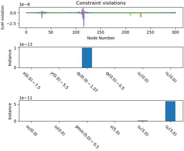
Plot the constraint violations.

_ = prob.plot_constraint_violations(solution)

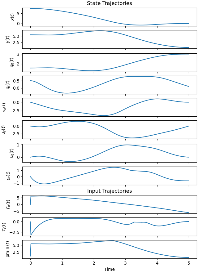
Plot generalized coordinates / speeds and forces / torques

_ = prob.plot_trajectories(solution)

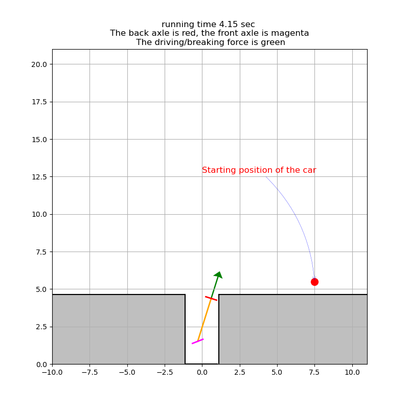
Animate the Car

The green arrow symbolizes the force which opty calculated to drive the car. It is perpendicular to the rear axle.

fps = 17


def add_point_to_data(line, x, y):
    # to trace the path of the point. Copied from Timo.
    old_x, old_y = line.get_data()
    line.set_data(np.append(old_x, x), np.append(old_y, y))


state_vals, input_vals, _ = prob.parse_free(solution)
t_arr = prob.time_vector()
state_sol = CubicSpline(t_arr, state_vals.T)
input_sol = CubicSpline(t_arr, input_vals.T)

# create additional points for the axles
Pbl, Pbr, Pfl, Pfr = sm.symbols('Pbl Pbr Pfl Pfr', cls=me.Point)

# end points of the force, length of the axles
Fbq = me.Point('Fbq')
la = sm.symbols('la')
fb, tq = sm.symbols('f_b, t_q')

Pbl.set_pos(Pb, -la/2 * Ab.x)
Pbr.set_pos(Pb, la/2 * Ab.x)
Pfl.set_pos(Pf, -la/2 * Af.x)
Pfr.set_pos(Pf, la/2 * Af.x)

Fbq.set_pos(Pb, fb * Ab.y)

coordinates = Pb.pos_from(O).to_matrix(N)
for point in (Dmc, Pf, Pbl, Pbr, Pfl, Pfr, Fbq):
    coordinates = coordinates.row_join(point.pos_from(O).to_matrix(N))

pL, pL_vals = zip(*par_map.items())
la1 = par_map[l] / 4.                      # length of an axle
la2 = la1/2.0
coords_lam = sm.lambdify((*state_symbols, fb, tq, pmin, *pL, la), coordinates,
                         cse=True)


def init():
    # needed to give the picture the right size.
    xmin, xmax = -10, 11.
    ymin, ymax = 0.0, 21.

    fig = plt.figure(figsize=(8, 8))
    ax = fig.add_subplot(111)
    ax.set_xlim(xmin, xmax)
    ax.set_ylim(ymin, ymax)
    ax.set_aspect('equal')
    ax.grid()

    ax.plot(7.5, 5.5, 'ro', markersize=10)
    ax.plot((par_map[x1]-la2, par_map[x1]-la2), (0.0, par_map[y12]-la2),
            color='black', lw=1.5)
    ax.plot((par_map[x2]+la2, par_map[x2]+la2), (0.0, par_map[y12]-la2),
            color='black', lw=1.5)
    ax.plot((xmin, par_map[x1]-la2), (par_map[y12]-la2, par_map[y12]-la2),
            color='black', lw=1.5)
    ax.plot((par_map[x2]+la2, xmax), (par_map[y12]-la2, par_map[y12]-la2),
            color='black', lw=1.5)
    ax.plot((par_map[x1]-la2, par_map[x2]+0.25), (0.0, 0.0),
            color='black', lw=1.5)

    ax.fill_between((xmin, par_map[x1]-la2), (par_map[y12]-la2,
                    par_map[y12]-la2), color='grey', alpha=0.5)
    ax.fill_between((par_map[x2]+la2, xmax), (par_map[y12]-la2,
                    par_map[y12]-la2), color='grey', alpha=0.5)

    ax.annotate('Starting position of the car',
                xy=(7.5, 5.5),
                arrowprops=dict(arrowstyle='->',
                                connectionstyle='arc3, rad=-.2',
                                lw=0.25, color='blue'),
                xytext=(0.0, 12.75), fontsize=12, color='red')

    # Initialize the block
    line1, = ax.plot([], [], color='orange', lw=2)
    line2, = ax.plot([], [], color='red', lw=2)
    line3, = ax.plot([], [], color='magenta', lw=2)
    line4 = ax.quiver([], [], [], [], color='green', scale=35,
                      width=0.004, headwidth=8)

    return fig, ax, line1, line2, line3, line4


# Function to update the plot for each animation frame
fig, ax, line1, line2, line3, line4 = init()


def update(t):
    message = (f'running time {t:.2f} sec \n The back axle is red, the '
               f'front axle is magenta \n The driving/breaking force is green')
    ax.set_title(message, fontsize=12)

    coords = coords_lam(*state_sol(t), *input_sol(t), *pL_vals, la1)

    #   Pb, Dmc, Pf, Pbl, Pbr, Pfl, Pfr, Fbq
    line1.set_data([coords[0, 0], coords[0, 2]], [coords[1, 0], coords[1, 2]])
    line2.set_data([coords[0, 3], coords[0, 4]], [coords[1, 3], coords[1, 4]])
    line3.set_data([coords[0, 5], coords[0, 6]], [coords[1, 5], coords[1, 6]])

    line4.set_offsets([coords[0, 0], coords[1, 0]])
    line4.set_UVC(coords[0, 7] - coords[0, 0], coords[1, 7] - coords[1, 0])

    return line1, line2, line3, line4,


frames = np.linspace(t0, tf, int(fps * (tf - t0)))
animation = FuncAnimation(fig, update, frames=frames, interval=1000 / fps)

Once Loop Reflect

A frame from the animation. sphinx_gallery_thumbnail_number = 4

fig, ax, line1, line2, line3, line4 = init()
update(4.15)

plt.show()