Car around Pylons

Objectives

• Show how to use inequality constrains for equations of motion

• Show how to come close to intermediate points on a solution path at times specified by opty.

Introduction

A car with rear wheel drive and front steering must move close to two points and return to its starting point. It can only move forward. The car is modeled as a rigid body with three bodies. The car is driven by a force at the rear axis and steered by a torque at the front axis. The acceleration is limited at the front and at the rear end of the car to avoid sliding off the road.

There is no speed allowed perpendicular to the wheels, realized by two velocity constraints. (The trajectories show, that the car is at the limit often, as one would expect if, as it is the case here, duration has to be minimized)

Method to Achieve the Objective

Make the car to come ‘close’ to two points, but without specifying the time when it should be there. opty should find the best time for the car to be there.

• Set the two points as \((x_{b_1}, y_{b_1})\) and \((x_{b_2}, y_{b_2})\) and an allowable ‘radius’ called epsilon around these points.

• Create a differentiable function \(\textrm{hump}(x, a, b, \textrm{steepness})\) such that it is one for \(a \leq x \leq b\) and zero otherwise. \(\textrm{steepness} > 0\) is a parameter that determines how ‘sharp’ the transition is, the larger the sharper.

• In order to know at the end of the run whether the car came close to the points during its course, integrate the hump function over time. These are the variables \(\textrm{punkt}_1, \textrm{punkt}_2\) with \(\textrm{punkt}_1 = \int_{t0}^{tf} \textrm{hump}(...) \, dt > 0\) if the car came close to the point, = 0 otherwise. Same for \(\textrm{punkt}_2\).

• The exact values of \(\textrm{punkt}_1, \textrm{punkt}_2\) are not known and should simply be positive ‘enough’, include two additional input trajectories \(\textrm{dist}_1, \textrm{dist}_2\) and specified variables \(h_1, h_2\).

• By setting \(\textrm{dist}_1 = \textrm{punkt}_1 \cdot h_1\) and \(\textrm{dist}_2 = \textrm{punkt}_2 \cdot h_2\) and bounding \(h_1, h_2 \in (1, \textrm{value})\), and setting \(\textrm{dist}_1(t_f) = 1\), one can ensure that \(\textrm{punkt}_1 > \dfrac{1}{\textrm{value}}\) and \(\textrm{punkt}_2 > \dfrac{1}{\textrm{value}}\).

States

• \(x, y\) : coordinates of front of the car

• \(u_x, u_y\) : velocity of the front of the car

• \(q_0\) : angle of the body of the car

• \(u_0\) : angular velocity of the body of the car

• \(q_f\) : angle of the front axis relative to the body

• \(u_f\) : angular velocity of the front axis relative to the body

• \(\textrm{punkt}_1, \textrm{punkt}_2\) : variables to ensure the car comes close to the points

Specifieds

• \(T_f\) : torque at the front axis, that is steering torque

• \(F_b\) : force at the rear axis, that is driving force

• \(h_1, h_2\) : variables to ensure the car comes close to the points

• \(\textrm{dist}_1, \textrm{dist}_2\) : variables to ensure the car comes close to the points

Known Parameters

• \(l\) : length of the car

• \(m_0\) : mass of the body of the car

• \(m_b\) : mass of the rear axis

• \(m_f\) : mass of the front axis

• \(iZZ_0\) : moment of inertia of the body of the car

• \(iZZ_b\) : moment of inertia of the rear axis

• \(iZZ_f\) : moment of inertia of the front axis

• \(\textrm{reibung}\) : friction coefficient between the car and the street

• \(x_{b_1}\) : x coordinate of pylon 1

• \(y_{b_1}\): y coordinate of pylon 1

• \(x_{b_2}\) : x coordinate of pylon 2

• \(y_{b_2}\): y coordinate of pylon 2

Unknown Parameters

• \(h\) : time step

import os
import sympy.physics.mechanics as me
import numpy as np
import sympy as sm
from scipy.interpolate import CubicSpline

from opty.direct_collocation import Problem
import matplotlib.pyplot as plt
from matplotlib.animation import FuncAnimation
from matplotlib.patches import Circle

Equations of Motion

N, A0, Ab, Af = sm.symbols('N A0 Ab Af', cls=me.ReferenceFrame)
t = me.dynamicsymbols._t
O, Pb, Dmc, Pf = sm.symbols('O Pb Dmc Pf', cls=me.Point)
O.set_vel(N, 0)

q0, qf = me.dynamicsymbols('q_0 q_f')
u0, uf = me.dynamicsymbols('u_0 u_f')
x, y = me.dynamicsymbols('x y')
ux, uy = me.dynamicsymbols('u_x u_y')
Tf, Fb = me.dynamicsymbols('T_f F_b')

reibung = sm.symbols('reibung')
l, m0, mb, mf, iZZ0, iZZb, iZZf = sm.symbols('l m0 mb mf iZZ0, iZZb, iZZf')

A0.orient_axis(N, q0, N.z)
A0.set_ang_vel(N, u0 * N.z)

Ab.orient_axis(A0, 0, N.z)

Af.orient_axis(A0, qf, N.z)
rot = Af.ang_vel_in(N)
Af.set_ang_vel(N, uf * N.z)
rot1 = Af.ang_vel_in(N)

Pf.set_pos(O, x * N.x + y * N.y)
Pf.set_vel(N, ux * N.x + uy * N.y)

Pb.set_pos(Pf, -l * A0.y)
Pb.v2pt_theory(Pf, N, A0)

Dmc.set_pos(Pf, -l/2 * A0.y)
Dmc.v2pt_theory(Pf, N, A0)
prevent_print = 1

No speed perpendicular to the wheels.

vel1 = me.dot(Pb.vel(N), Ab.x) - 0
vel2 = me.dot(Pf.vel(N), Af.x) - 0

Dynamic equations of motion, Kane’s method.

I0 = me.inertia(A0, 0, 0, iZZ0)
body0 = me.RigidBody('body0', Dmc, A0, m0, (I0, Dmc))
Ib = me.inertia(Ab, 0, 0, iZZb)
bodyb = me.RigidBody('bodyb', Pb, Ab, mb, (Ib, Pb))
If = me.inertia(Af, 0, 0, iZZf)
bodyf = me.RigidBody('bodyf', Pf, Af, mf, (If, Pf))
bodies = [body0, bodyb, bodyf]

forces = [(Pb, Fb * Ab.y), (Af, Tf * N.z), (Dmc, -reibung * Dmc.vel(N))]

kd = sm.Matrix([ux - x.diff(t), uy - y.diff(t), u0 - q0.diff(t),
                me.dot(rot1 - rot, N.z)])
speed_constr = sm.Matrix([vel1, vel2])

q_ind = [x, y, q0, qf]
u_ind = [u0, uf]
u_dep = [ux, uy]

KM = me.KanesMethod(
    N,
    q_ind=q_ind,
    u_ind=u_ind,
    kd_eqs=kd,
    u_dependent=u_dep,
    velocity_constraints=speed_constr,
)
(fr, frstar) = KM.kanes_equations(bodies, forces)
eom = fr + frstar
eom = kd.col_join(eom)
eom = eom.col_join(speed_constr)

Constraints so the car approaches the points \((x_{b_1}, y_{b_1})\), and \((x_{b_2}, y_{b_2})\) at whatever times opty chooses, explanation above. Also here it is enforced that it can only move forward. If steepness is large optimazation will not work it may become too ‘non-differentiable’.

steepness = sm.symbols('steepness')


def hump(x, a, b, steepness):
    # approx one for x in [a, b]
    # approx zero otherwise
    # the higher steepness the closer the approximation
    res = 1.0 - (1 / (1 + sm.exp(steepness*(x - a)))
                 + 1 / (1 + sm.exp(-steepness * (x - b))))
    return res


punkt1, punkt2 = me.dynamicsymbols('punkt1 punkt2')
dist1, dist2 = me.dynamicsymbols('dist1 dist2')
h1, h2 = me.dynamicsymbols('h1 h2')

xb1, yb1, xb2, yb2 = sm.symbols('xb yb xb2 yb2')
epsilon = sm.symbols('epsilon')

treffer1 = (hump(x, xb1-epsilon, xb1+epsilon, 5)*hump(y, yb1-epsilon,
                                                      yb1+epsilon, steepness))
treffer2 = (hump(x, xb2-epsilon, xb2+epsilon, 5)*hump(y, yb2-epsilon,
                                                      yb2+epsilon, steepness))

eom_add = sm.Matrix([
    -punkt1.diff(t) + treffer1,
    -punkt2.diff(t) + treffer2,
    -dist1 + punkt1 * h1,
    -dist2 + punkt2 * h2,
])

eom = eom.col_join(eom_add)

Acceleration constraints, so the car does not slide off the road. Constraint so the care only moves forward.

forward = Pb.vel(N).dot(Ab.y)
accel_front = Pf.acc(N).dot(A0.x)
accel_back = Pb.acc(N).dot(A0.x)
beschleunigung = sm.Matrix([forward, accel_front, accel_back])

eom = eom.col_join(beschleunigung)

print(f'eom too large to print out. Its shape is {eom.shape} and it has '
      f'{sm.count_ops(eom)} operations')

eom too large to print out. Its shape is (15, 1) and it has 555 operations

Set up the Optimization Problem and Solve It

h = sm.symbols('h')
state_symbols = ([x, y, q0, qf, ux, uy, u0, uf] +
                 [punkt1, punkt2])
constant_symbols = (l, m0, mb, mf, iZZ0, iZZb, iZZf, reibung)
specified_symbols = (Fb, Tf, h1, h2, dist1, dist2)

num_nodes = 401
t0 = 0.0
interval_value = h
tf = h * (num_nodes - 1)

Specify the known system parameters.

par_map = {}
par_map[m0] = 1.0
par_map[mb] = 0.5
par_map[mf] = 0.5
par_map[iZZ0] = 1.
par_map[iZZb] = 0.5
par_map[iZZf] = 0.5
par_map[l] = 3.0
par_map[reibung] = 0.5
par_map[xb1] = 10.0
par_map[yb1] = 15.0
par_map[xb2] = -5.0
par_map[yb2] = 10.0
par_map[epsilon] = 0.5
par_map[steepness] = 5.0

Define the objective function and its gradient. The time needed is to be minimized.

def obj(free):
    return free[-1]


def obj_grad(free):
    grad = np.zeros_like(free)
    grad[-1] = 1.0
    return grad

Set up the constraints, the bounds and the Problem.

instance_constraints = (
    x.func(t0),
    y.func(t0),
    q0.func(t0),
    ux.func(t0),
    uy.func(t0),
    u0.func(t0),
    uf.func(t0),
    punkt1.func(t0),
    punkt2.func(t0),
    dist1.func(t0),
    dist2.func(t0),
    x.func(tf),
    y.func(tf),
    ux.func(tf),
    uy.func(tf),
    dist1.func(tf) - 1.0,
    dist2.func(tf) - 1.0,
)

grenze = 20.0
grenze1 = 5.0
delta = np.pi/4.0
bounds = {
    Fb: (-grenze, grenze),
    Tf: (-grenze, grenze),
    # restrict the steering angle
    qf: (-np.pi/2. + delta - 1.e-5, np.pi/2. - delta + 1.e-5),
    x: (-20, 20),
    y: (-15, 30),
    h: (0.0, 0.5),
    h1: (1.0, 5.0),
    h2: (1.0, 5.0),
}

eom_bounds = {
    12: (0.0, np.inf),
    13: (-grenze1, grenze1),
    14: (-grenze1, grenze1),
}

prob = Problem(
    obj,
    obj_grad,
    eom,
    state_symbols,
    num_nodes,
    interval_value,
    known_parameter_map=par_map,
    instance_constraints=instance_constraints,
    bounds=bounds,
    eom_bounds=eom_bounds,
    time_symbol=t,
    backend='numpy',
)

For the initial guess the result of some previous run is used to expedite execution, if available.

fname = f'car_around_pylons_{num_nodes}_nodes_solution.csv'
if os.path.exists(fname):
    # A result is available.
    solution = np.loadtxt(fname)
else:
    # No result is available, calculate a solution.
    np.random.seed(123)
    prob.add_option('max_iter', 6000)
    initial_guess = np.random.randn(prob.num_free)
    section = int(num_nodes/3)
    x1 = np.linspace(0.0, par_map[xb1], section)
    y1 = np.linspace(0.0, par_map[yb1], section)
    x2 = np.linspace(par_map[xb1], par_map[xb2], section)
    y2 = np.linspace(par_map[yb1], par_map[yb2], section)
    x3 = np.linspace(par_map[xb2], 0.0, section)
    y3 = np.linspace(par_map[yb2], 0.0, section)
    xges = np.concatenate((x1, x2, x3))
    yges = np.concatenate((y1, y2, y3))
    initial_guess[0:3*section] = xges
    initial_guess[3*section:6*section] = yges
    for i in range(5):
        print(f'{i+1} - th iteration')
        solution, info = prob.solve(initial_guess)
        initial_guess = solution

        print('message from optimizer:', info['status_msg'])
        print('Iterations needed', len(prob.obj_value))
        print(f"objective value {info['obj_val']:.3e} \n")

    _ = prob.plot_objective_value()

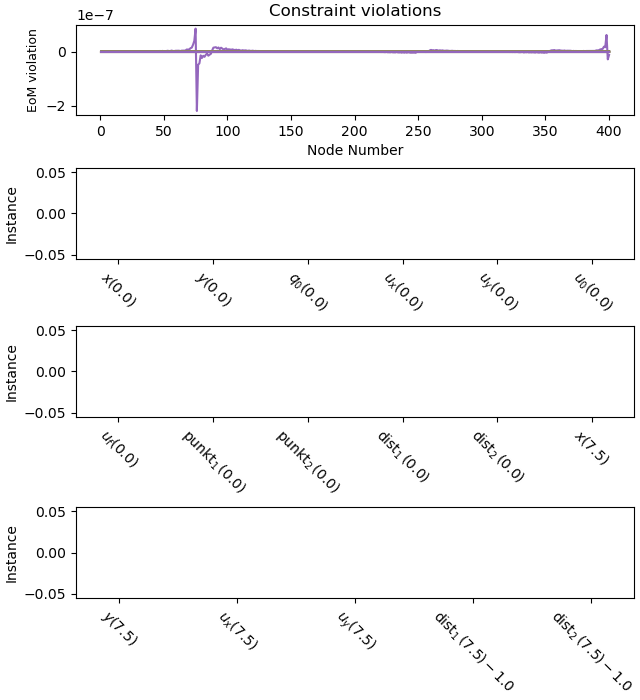
Plot the constraint violations.

_ = prob.plot_constraint_violations(solution, subplots=False)

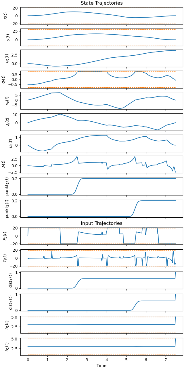
Plot generalized coordinates / speeds and forces / torques

_ = prob.plot_trajectories(solution, show_bounds=True)

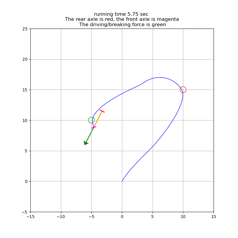
Animate the Car

fps = 10

state_vals, input_vals, _, h_val = prob.parse_free(solution)

tf = h_val*(num_nodes - 1)
t_arr = prob.time_vector(solution=solution)
state_sol = CubicSpline(t_arr, state_vals.T)
input_sol = CubicSpline(t_arr, input_vals.T)

# create additional points for the axles
Pbl, Pbr, Pfl, Pfr = sm.symbols('Pbl Pbr Pfl Pfr', cls=me.Point)

# end points of the force, length of the axles
Fbq = me.Point('Fbq')
la = sm.symbols('la')
fb, tq = sm.symbols('f_b, t_q')

Pbl.set_pos(Pb, -la/2 * Ab.x)
Pbr.set_pos(Pb, la/2 * Ab.x)
Pfl.set_pos(Pf, -la/2 * Af.x)
Pfr.set_pos(Pf, la/2 * Af.x)

Fbq.set_pos(Pb, fb * Ab.y)

coordinates = Pb.pos_from(O).to_matrix(N)
for point in (Dmc, Pf, Pbl, Pbr, Pfl, Pfr, Fbq):
    coordinates = coordinates.row_join(point.pos_from(O).to_matrix(N))

pL, pL_vals = zip(*par_map.items())
la1 = par_map[l] / 4.                      # length of an axle

coords_lam = sm.lambdify((*state_symbols, fb, tq, *pL, la), coordinates,
                         cse=True)


def init():
    xmin, xmax = -15, 15.
    ymin, ymax = -5, 25.

    fig = plt.figure(figsize=(8, 8))
    ax = fig.add_subplot(111)
    ax.set_xlim(xmin, xmax)
    ax.set_ylim(ymin, ymax)
    ax.set_aspect('equal')
    ax.grid()
    circle1 = Circle((par_map[xb1], par_map[yb1]), par_map[epsilon],
                     edgecolor='red', facecolor='none', linewidth=1)
    ax.add_patch(circle1)
    circle2 = Circle((par_map[xb2], par_map[yb2]), par_map[epsilon],
                     edgecolor='green', facecolor='none', linewidth=1)
    ax.add_patch(circle2)

    line1, = ax.plot([], [], color='orange', lw=2)
    line2, = ax.plot([], [], color='red', lw=2)
    line3, = ax.plot([], [], color='magenta', lw=2)
    line4 = ax.quiver([], [], [], [], color='green', scale=35, width=0.004,
                      headwidth=8)
    line5, = ax.plot([], [], color='blue', lw=1)

    return fig, ax, line1, line2, line3, line4, line5


fig, ax, line1, line2, line3, line4, line5 = init()

zeiten = np.linspace(t0, tf, int(fps * (tf - t0)))


def update(t):
    message = (f'running time {t:.2f} sec \n The rear axle is red, the '
               f'front axle is magenta \n The driving/breaking force is green')
    ax.set_title(message, fontsize=12)

    coords = coords_lam(*state_sol(t), input_sol(t)[0], input_sol(t)[1],
                        *pL_vals, la1)

    koords = []
    for zeit in zeiten:
        koords.append(coords_lam(*state_sol(zeit), input_sol(zeit)[0],
                                 input_sol(zeit)[1], *pL_vals, la))

    line1.set_data([coords[0, 0], coords[0, 2]], [coords[1, 0], coords[1, 2]])
    line2.set_data([coords[0, 3], coords[0, 4]], [coords[1, 3], coords[1, 4]])
    line3.set_data([coords[0, 5], coords[0, 6]], [coords[1, 5], coords[1, 6]])

    line4.set_offsets([coords[0, 0], coords[1, 0]])
    line4.set_UVC(coords[0, 7] - coords[0, 0], coords[1, 7] - coords[1, 0])

    zaehler1 = np.argwhere(zeiten >= t)[0][0] + 1
    line5.set_data([koords[i][0, 2] for i in range(zaehler1)],
                   [koords[i][1, 2] for i in range(zaehler1)])


frames = np.linspace(t0, tf, int(fps*(tf - t0)))
animation = FuncAnimation(fig, update, frames=frames, interval=1000/fps)

Once Loop Reflect

fig, ax, line1, line2, line3, line4, line5 = init()
update(5.75)

plt.show()