Note
Go to the end to download the full example code.
Ball Rolling on Spinning Disc
Objectives
Shows an objective function that is a weighted sum of energy and speed.
Shows how to go about if one wants to calculate the reaction forces in addition to finding the optimal solution, without setting up the equations of motion twice.
Introduction
A uniform, solid ball with radius \(r\) and mass \(m_b\) is rolling on a horizontal spinning disc without slipping. The disc starts at rest and speeds up like this
where
\(\alpha > 0\) is a measure of the acceleration and
\(\Omega\) is the final rotational speed.
A torque is applied to the ball, and the goal is to get it to the center of the disc.
An observer, a particle of mass \(m_o\), is attached to the surface the ball.
Constants
\(m_b\): mass of the ball [kg]
\(r\) : radius of the ball [m]
\(m_o\) : mass of the observer [kg]
\(\Omega\): final rotational speed of the disc around [rad/sec]
\(\alpha\): measure of the acceleration of the disc [1/sec]
States
\(q_1, q_2, q_3\): generalized coordinates of the ball w.r.t the disc [rad]
\(u_1, u_2, u_3\): generalized angual velocities of the ball [rad/sec]
Specifieds
\(t_1, t_2, t_3\): Torque applied to the ball [N * m]
Additional parameters
\(N\) inertial frame
\(A_1\): frame fixed to the ball
\(A_2\): frame fixed to the disc
\(O\): point fixed in N
\(C_P\): contact point of ball with disc
\(A^{o}_1\): center of mass of the ball
\(pos_\textrm{observer}\): position of the observer
\(h\): interval which opty should minimize.
This example was inspired by the demonstration by Steve Mould:
import os
from matplotlib import patches
from matplotlib.animation import FuncAnimation
from opty.direct_collocation import Problem
from scipy.interpolate import CubicSpline
from scipy.optimize import root
import matplotlib.pyplot as plt
import numpy as np
import sympy as sm
import sympy.physics.mechanics as me
Set up the Equations of Motion
Initialize the variables.
t = me.dynamicsymbols._t
q1, q2, q3 = me.dynamicsymbols('q1 q2 q3')
u1, u2, u3 = me.dynamicsymbols('u1 u2 u3')
x, y, ux, uy = me.dynamicsymbols('x, y, ux, uy')
t1, t2, t3 = me.dynamicsymbols('t1 t2 t3')
rhs = list(sm.symbols('rhs:5'))
aux = me.dynamicsymbols('auxx, auxy, auxz')
F_r = me.dynamicsymbols('Fx, Fy, Fz')
# Introduce a variable to mimick the time. This is a hack, as opty does not yet
# support time being explicit in the equations of motion.
T = sm.symbols('T', cls=sm.Function)
Tdot, Tdotdot = sm.symbols('Tdot Tdotdot')
mb, mo, g, r = sm.symbols('mb, mo, g, r')
Omega, alpha = sm.symbols('Omega, alpha')
N, A1, A2 = sm.symbols('N, A1 A2', cls=me.ReferenceFrame)
O, CP, Ao1, pos_observer = sm.symbols('O, CP, Ao1, pos_observer', cls=me.Point)
O.set_vel(N, 0)
Determination of the holonomic constraints.
If the ball rotates around the x axis by an angle \(q_1\) the contact point will be move by \(-q_1 r\) in the \(\hat{A_2}_y\) direction. If the ball rotates around the y axis by an angle \(q_2\) the contact point will be move by \(q_2 r\) in the \(\hat{A_2}_x\) direction. Hence the configuration constraints are:
\(x = r q_2\)
\(y = -r q_1\)
So the resulting speed constraints are:
\(\dfrac{d}{dt}(x) = r \dfrac{d}{dt}(q_2)\)
\(\dfrac{d}{dt}(y) = -r \dfrac{d}{dt}(q_1)\)
The time \(t\) appears explicitly in the EOMs. So, declare a function \(T(t)\), and then pass the time as known trajectory. The EOMs also contain \(\dfrac{d}{dt}(T(t))\) and \(\dfrac{d^2}{dt^2}(T(t))\) As \(T(t) = const \cdot t\) the derivatives accordingly are set accordingly.
qdisc = sm.integrate(udisc, t) is not used, as this gives a
sm.Piecewise(..) result, likely not differentiable everywhere, but
the result of this integration is still used for \(\alpha \neq 0\).
udisc = Omega*(1 - sm.exp(-alpha*T(t)))
qdisc = (Omega*T(t) + Omega*sm.exp(-alpha*T(t))/alpha - Omega/alpha)
A2.orient_axis(N, qdisc, N.z)
A2.set_ang_vel(N, udisc*N.z)
A1.orient_body_fixed(A2, (q1, q2, q3), '123')
rot = A1.ang_vel_in(N)
A1.set_ang_vel(A2, u1*A1.x + u2*A1.y + u3*A1.z)
rot1 = A1.ang_vel_in(N)
CP.set_pos(O, x*A2.x + y*A2.y)
CP.set_vel(A2, ux*A2.x + uy*A2.y)
Ao1.set_pos(CP, r*N.z)
Ao1.set_vel(N, Ao1.pos_from(O).diff(t, N) + aux[0]*N.x + aux[1]*N.y +
aux[2]*N.z)
pos_observer.set_pos(Ao1, r*A1.x)
pos_observer.v2pt_theory(Ao1, N, A1)
iXX = 2./5. * mb * r**2
iYY = iXX
iZZ = iXX
I = me.inertia(A1, iXX, iYY, iZZ)
ball = me.RigidBody('ball', Ao1, A1, mb, (I, Ao1))
observer = me.Particle('observer', pos_observer, mo)
bodies = [ball, observer]
forces = [(Ao1, -mb*g*N.z + F_r[0]*N.x + F_r[1]*N.y + F_r[2]*N.z),
(pos_observer, -mo*g*N.z), (A1, t1*A1.x + t2*A1.y + t3*A1.z)]
kd = sm.Matrix([ux - x.diff(t), uy - y.diff(t),
*[(rot - rot1).dot(uv) for uv in N]])
speed_constr = sm.Matrix([ux - r*u2, uy + r*u1])
hol_constr = sm.Matrix([x - r*q2, y + r*q1])
q_ind = [q1, q2, q3]
q_dep = [x, y]
u_ind = [u1, u2, u3]
u_dep = [ux, uy]
KM = me.KanesMethod(
N,
q_ind=q_ind,
q_dependent=q_dep,
u_ind=u_ind,
u_dependent=u_dep,
u_auxiliary=aux,
kd_eqs=kd,
velocity_constraints=speed_constr,
configuration_constraints=hol_constr,
)
Set the equations of motion needed to calculate the reaction forces.
fr, frstar = KM.kanes_equations(bodies, forces)
MM = KM.mass_matrix_full
force = me.msubs(KM.forcing_full,
{sm.Derivative(T(t), t): Tdot, sm.Derivative(T(t), (t, 2)):
Tdotdot}, {i: 0 for i in F_r})
react_forces = me.msubs(KM.auxiliary_eqs,
{sm.Derivative(T(t), t):
Tdot, sm.Derivative(T(t), (t, 2)): 0},
{i.diff(t): rhs[j] for j, i in enumerate(u_ind +
u_dep)})
Modify the equations of motion for the optimization problem. So the last three equations, corresponding to the reaction forces \(F_x, F_y, F_z\) are removed. As the remaining three equation also contain \(F_x, F_y, F_z\) they are set to zero.
frfrstar_reduced = me.msubs(sm.Matrix([(fr + frstar)[j] for j in range(3)]),
{i: 0 for i in F_r})
eom = kd.col_join(frfrstar_reduced)
eom = me.msubs((eom.col_join(hol_constr)), {sm.Derivative(T(t), t): Tdot,
sm.Derivative(T(t), (t, 2)):
Tdotdot},)
print(f'The equations of motion for the optinization contain '
f'{sm.count_ops(eom):,} operations, and shape {eom.shape}')
The equations of motion for the optinization contain 314,946 operations, and shape (10, 1)
Set Up the Optimization Problem and Solve It
h = sm.symbols('h')
state_symbols = (q1, q2, q3, x, y, u1, u2, u3, ux, uy)
laenge = len(state_symbols)
constant_symbols = (r, mb, mo, g, Omega, alpha, Tdot, Tdotdot)
specified_symbols = (t1, t2, t3)
num_nodes = 250
duration = (num_nodes - 1) * h
t0, tf = 0.0, duration
Disc time is the final time of \(T(t)\). Ideally it would be (num_nodes
- 1)*h, but it is not possible to use the result of the optimization as
input of a known trajectory. It is simply set to 7.5 sec.
disc_time = 7.5
interval_value = h
interval_value_fix = disc_time/num_nodes
interval_fix = np.linspace(0, disc_time, num_nodes)
Specify the known system parameters.
par_map = {}
par_map[mb] = 5.0
par_map[mo] = 1.0
par_map[r] = 1.0
par_map[Omega] = 10.0
par_map[alpha] = 0.5
par_map[g] = 9.81
par_map[Tdot] = interval_value_fix
par_map[Tdotdot] = 0.0
A weighted sum of energy and speed is to be minimized. weight is the
relative weight of the speed, weight > 0.
weight = 2.5e5
Define the objective function and its gradient. They are the sums of the objective function to minimize the energy and the objective function to minimize the speed. Same with the gradients.
def obj(free):
free1 = free[0: -1]
Tz1 = free1[laenge * num_nodes: (laenge + 1) * num_nodes]
Tz2 = free1[(laenge + 1) * num_nodes: (laenge + 2) * num_nodes]
Tz3 = free1[(laenge + 2) * num_nodes: (laenge + 3) * num_nodes]
return (free[-1] * (np.sum(Tz1**2) + np.sum(Tz2**2) + np.sum(Tz3**2)) +
free[-1] * weight)
def obj_grad(free):
grad = np.zeros_like(free)
grad[laenge*num_nodes: (laenge + 1)*num_nodes] = (
2.0*free[-1] *free[laenge*num_nodes: (laenge + 1)*num_nodes])
grad[(laenge + 1)*num_nodes: (laenge + 2)*num_nodes] = (
2.0*free[-1]*free[(laenge + 1)*num_nodes: (laenge + 2)*num_nodes])
grad[(laenge + 2)*num_nodes: (laenge + 3)*num_nodes] = (
2.0*free[-1]*free[(laenge + 2)*num_nodes: (laenge + 3)*num_nodes])
grad[-1] = weight
return grad
The initial state must satisfy the holonomic constraints.
x_start = 7.0
q2_start = x_start/par_map[r]
y_start = 7.0
q1_start = -y_start/par_map[r]
initial_state_constraints = {
q1: q1_start,
q2: q2_start,
q3: 0.0,
u1: 0.0,
u2: 0.0,
u3: 0.0,
x: x_start,
y: y_start,
ux: 0.0,
uy: 0.0
}
final_state_constraints = {
x: 0.0,
y: 0.0,
ux: 0.0,
uy: 0.0,
}
instance_constraints = (
q1.subs({t: t0}) - initial_state_constraints[q1],
q2.subs({t: t0}) - initial_state_constraints[q2],
q3.subs({t: t0}) - initial_state_constraints[q3],
u1.subs({t: t0}) - initial_state_constraints[u1],
u2.subs({t: t0}) - initial_state_constraints[u2],
u3.subs({t: t0}) - initial_state_constraints[u3],
x.subs({t: t0}) - initial_state_constraints[x],
y.subs({t: t0}) - initial_state_constraints[y],
ux.subs({t: t0}) - initial_state_constraints[ux],
uy.subs({t: t0}) - initial_state_constraints[uy],
x.subs({t: tf}) - final_state_constraints[x],
y.subs({t: tf}) - final_state_constraints[y],
ux.subs({t: tf}) - final_state_constraints[ux],
uy.subs({t: tf}) - final_state_constraints[uy],
)
Forcing h > 0 helps to avoid negative h solutions.
torque_limits = 10.0
bounds = {
t1: (-torque_limits, torque_limits),
t2: (-torque_limits, torque_limits),
t3: (-torque_limits, torque_limits),
h: (0.0, 1.0),
}
Create an optimization problem.
prob = Problem(
obj,
obj_grad,
eom,
state_symbols,
num_nodes,
interval_value,
known_parameter_map=par_map,
known_trajectory_map={T(t): interval_fix},
instance_constraints=instance_constraints,
time_symbol=t,
bounds=bounds,
)
Set up an initial guess and solve the problem, unless a solution file is already present.
fname = f'ball_rolling_on_spinning_disc_{num_nodes}_nodes_solution.csv'
if os.path.isfile(fname):
# solution available
solution = np.loadtxt(fname)
else:
# Set up a reasonable initial guess and solve the problem
i1b = np.zeros(num_nodes)
i2 = np.linspace(initial_state_constraints[x], final_state_constraints[x],
num_nodes)
i1a = i2/par_map[r]
i3 = np.linspace(initial_state_constraints[y], final_state_constraints[y],
num_nodes)
i1 = -i3/par_map[r]
i4 = np.zeros(8*num_nodes)
initial_guess = np.hstack((i1, i1a, i1b, i2, i3, i4, 0.01))
# This way the maximum number of interations may be changed. Default is
# 3000.
prob.add_option('max_iter', 1000)
# Find the optimal solution.
for _ in range(3):
solution, info = prob.solve(initial_guess)
initial_guess = solution
print('message from optimizer:', info['status_msg'])
print('Iterations needed', len(prob.obj_value))
print(f'Optimal h = {solution[-1]:.3e} sec')
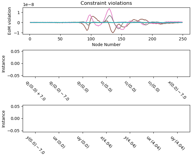
Plot the accuracy of the results.
_ = prob.plot_constraint_violations(solution)
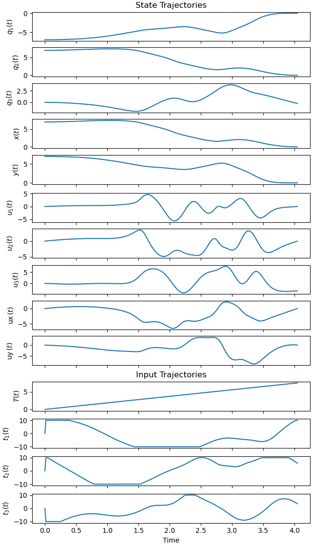
Plot the results.
_ = prob.plot_trajectories(solution)
Calculate and Plot the Reaction Forces
Convert the SymPy functions to NumPy functions.
qL = q_ind + q_dep + u_ind + u_dep + [T(t)] + [t1, t2, t3]
rhs = list(sm.symbols('rhs:5'))
pL = [i for i in par_map.keys()]
pL_vals = [par_map[i] for i in pL]
MM_lam = sm.lambdify(qL + pL, MM, cse=True)
force_lam = sm.lambdify(qL + pL, force, cse=True)
react_forces_lam = sm.lambdify(F_r + qL + pL + rhs, react_forces, cse=True)
state_vals, input_vals, _, h_val = prob.parse_free(solution)
resultat2 = state_vals.T
schritte2 = resultat2.shape[0]
Numerically find \(rhs_1 = MM^{-1} \cdot forces\) for the results found by the optimization.
times2 = interval_fix
rhs1 = np.empty((schritte2, resultat2.shape[1]))
for i in range(schritte2):
zeit1 = times2[i]
t11, t21, t31 = input_vals.T[i, :]
rhs1[i, :] = np.linalg.solve(
MM_lam(*[resultat2[i, j] for j in range(resultat2.shape[1])], zeit1,
t11, t21, t31, *pL_vals),
force_lam(*[resultat2[i, j] for j in range(resultat2.shape[1])], zeit1,
t11, t21, t31, *pL_vals)).reshape(10)
Numerically solve react_force for the reaction forces.
def func(x, *args):
return react_forces_lam(*x, *args).reshape(3)
forcex = np.empty(schritte2)
forcey = np.empty(schritte2)
forcez = np.empty(schritte2)
x0 = tuple((1., 1., 1.))
for i in range(schritte2):
y0 = [resultat2[i, j] for j in range(resultat2.shape[1])]
rhs = [rhs1[i, j] for j in range(5, 10)]
t11, t21, t31 = input_vals.T[i, :]
zeit1 = times2[i]
args = tuple(y0 + [zeit1, t11, t21, t31] + pL_vals + rhs)
AAA = root(func, x0, args=args)
forcex[i] = AAA.x[0]
forcey[i] = AAA.x[1]
forcez[i] = AAA.x[2]
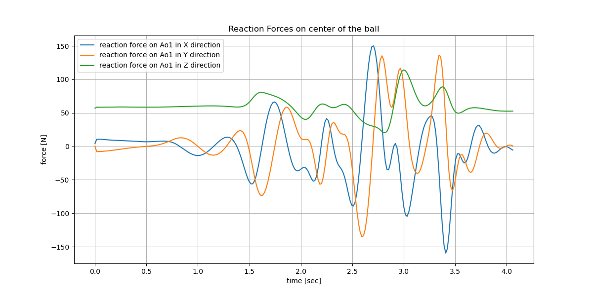
Plot the reaction forces.
times2 = interval_fix*h_val/interval_value_fix
fig, ax = plt.subplots(figsize=(12, 6))
for i, j in zip((forcex, forcey, forcez),
('reaction force on Ao1 in X direction',
'reaction force on Ao1 in Y direction',
'reaction force on Ao1 in Z direction')):
plt.plot(times2, i, label=j)
ax.set_title('Reaction Forces on center of the ball')
ax.set_xlabel('time [sec]')
ax.set_ylabel('force [N]')
ax.grid(True)
_ = ax.legend()
Animate the system.
fps = 30
def add_point_to_data(line, x, y):
old_x, old_y = line.get_data()
line.set_data(np.append(old_x, x), np.append(old_y, y))
state_vals, input_vals, _, h_val = prob.parse_free(solution)
t_arr = prob.time_vector(solution=solution)
state_sol = CubicSpline(t_arr, state_vals.T)
input_sol = CubicSpline(t_arr, input_vals.T)
x_max = np.max(np.max([np.abs(state_vals[3, i])for i in range(num_nodes)]))
y_max = np.max(np.max([np.abs(state_vals[4, i])for i in range(num_nodes)]))
r_disc = np.sqrt(x_max**2 + y_max**2) * 1.2
t1h, t2h, t3h = sm.symbols('t1h t2h t3h')
Pl, Pr, Pu, Pd, T_total, T_Z = sm.symbols('Pl Pr Pu Pd, T_total, T_Z',
cls=me.Point)
Pl.set_pos(O, -r_disc*A2.x)
Pr.set_pos(O, r_disc*A2.x)
Pu.set_pos(O, r_disc*A2.y)
Pd.set_pos(O, -r_disc*A2.y)
T_total.set_pos(Ao1, t1h*A1.x + t2h*A1.y + t3h*A1.z)
The projection of the total torque onto the X/Y plane is shown. Is vertical component is shown, somewhat arbitrarily, as perpendicular to the projection.
hilfs = sm.Max(t1h**2 + t2h**2 + t3h**2, 1.e-15)
x_coord = (t1h*A1.x + t2h*A1.y + t3h*A1.z).dot(A2.x)
y_coord = (t1h*A1.x + t2h*A1.y + t3h*A1.z).dot(A2.y)
T_Z.set_pos(Ao1, t3h/sm.sqrt(hilfs) * (y_coord*A2.x - x_coord*A2.y))
coordinates = Ao1.pos_from(O).to_matrix(N)
for point in (pos_observer, Pl, Pr, Pu, Pd, T_total, T_Z):
coordinates = coordinates.row_join(point.pos_from(O).to_matrix(N))
pL, pL_vals = zip(*par_map.items())
coords_lam = sm.lambdify(list(state_symbols) + [t1h, t2h, t3h] + list(pL) +
[T(t)], coordinates, cse=True)
old_x, old_y = [], []
def init_plot():
fig, ax = plt.subplots(figsize=(6, 6), layout='constrained')
ax.set_xlim(-r_disc-1, r_disc+1)
ax.set_ylim(-r_disc-1, r_disc+1)
ax.set_aspect('equal')
ax.set_xlabel('x', fontsize=15)
ax.set_ylabel('y', fontsize=15)
# draw the spokes
line1, = ax.plot([], [], lw=2, marker='o', markersize=0, color='black')
line2, = ax.plot([], [], lw=2, marker='o', markersize=0, color='black')
line3, = ax.plot([], [], lw=2, marker='o', markersize=0, color='black')
line4, = ax.plot([], [], lw=2, marker='o', markersize=0, color='black')
# draw the path of the ball.
line5, = ax.plot([], [], color='magenta', lw=0.5)
# draw the torque vektor
pfeil1 = ax.quiver([], [], [], [], color='green', scale=30, width=0.004)
pfeil2 = ax.quiver([], [], [], [], color='blue', scale=30, width=0.004)
# draw the ball
ball = patches.Circle((initial_state_constraints[x],
initial_state_constraints[y]), radius=par_map[r],
fill=True, color='magenta', alpha=0.75)
ax.add_patch(ball)
# draw the observer
observer, = ax.plot([], [], marker='o', markersize=5, color='blue')
return (fig, ax, line1, line2, line3, line4, line5, ball, observer, pfeil1,
pfeil2)
(fig, ax, line1, line2, line3, line4, line5,
ball, observer, pfeil1, pfeil2) = init_plot()
# draw the disc
phi = np.linspace(0, 2*np.pi, 500)
x_phi = r_disc * np.cos(phi)
y_phi = r_disc * np.sin(phi)
ax.plot(x_phi, y_phi, color='black', lw=2)
def update(t):
global old_x, old_y
message = (
f'running time {t:.2f} sec \n The green arrow is the '
f'projection of the torque vector on the X/Y plane \n'
f'The blue arrow is the component of the torque perpendicular '
f'to the disc \n'
f'The blue dot is the observer \n'
f'The magenta line is the path of the ball in the inertial frame'
)
ax.set_title(message, fontsize=10)
coords = coords_lam(*state_sol(t), *input_sol(t), *pL_vals, t)
line1.set_data([0, coords[0, 2]], [0, coords[1, 2]])
line2.set_data([0, coords[0, 3]], [0, coords[1, 3]])
line3.set_data([0, coords[0, 4]], [0, coords[1, 4]])
line4.set_data([0, coords[0, 5]], [0, coords[1, 5]])
old_x.append(coords[0, 0])
old_y.append(coords[1, 0])
add_point_to_data(line5, coords[0, 0], coords[1, 0])
observer.set_data([coords[0, 1]], [coords[1, 1]])
ball.set_center((coords[0, 0], coords[1, 0]))
pfeil1.set_offsets([coords[0, 0], coords[1, 0]])
pfeil1.set_UVC(coords[0, -2] - coords[0, 0], coords[1, -2] - coords[1, 0])
pfeil2.set_offsets([coords[0, 0], coords[1, 0]])
pfeil2.set_UVC(coords[0, -1] - coords[0, 0], coords[1, -1] - coords[1, 0])
return line1, line2, line3, line4, line5, ball, observer, pfeil1, pfeil2
animation = FuncAnimation(fig, update,
frames=np.arange(t0, (num_nodes - 1)*h_val,
1/fps),
interval=1000/fps, blit=False)