Note
Go to the end to download the full example code.
Particle Flight in Tube
Objectives
Shows how the introduction of an additional state variable may be used to solve a nonlinear equation. A state variable is used as its time derivative is needed.
Shows the use of inequalities constraints.
Introduction
A particle of mass \(m\) is moving from a starting point to an ending point, subject to a viscous friction force and to a uniform gravitational field. The particle must not leave a tube defined by a curve (centerline) in space and a radius. At one point during the motion, it must pass through a narrow gate, modelled as a circle.
Detailed Description on how the Objectives are Achieved
(In what follows all components are with respect to the inertial frame N.) The curve is given as \(X(r) = (f(r, \textrm{params}), g(r, \textrm{params}), h(r, \textrm{params}))\), where \(r\) is the parameter of the curve. Let \(\textrm{cut}_{\textrm{param}}\) be the parameter of the curve where the distance of the particle from the curve is closest. Then \(( \dfrac{df}{dr}, \dfrac{dg}{dr}, \dfrac{dh}{dr} ) |_{r = \textrm{cut}_{\textrm{param}}}\) is the tangential vector on the curve at the point of closest distance from the particle.
The equation of the plane, which is perpendicular to the curve at the point of closest distance and contains the point of the particle is formed. The intersection of the curve and the plane gives the point of closest distance of the curve from the particle. This leads to a nonlinear equation for \(\textrm{cut}_{\textrm{param}}\), which is added to the equations of motion by declaring a new state variable \(\textrm{cut}_{\textrm{param}}\).
The particle must not leave the tube with radius \(\textrm{radius}\). At a certain point on the curve, determined by \(\textrm{cut}_{\textrm{param}} = \textrm{wo}\), the paricle must pass through a narrow gate. the gate is modeled as a circle with its center on the curve, and with radius \(\textrm{radius} \cdot \textrm{factor}\), with \(0 < \textrm{factor} < 1\). This is accomplished with the help of a smooth hump function. This hump function equals one around a vicinity of \(\textrm{wo}\), determined by \(\epsilon\), and zero otherwise.
Notes
Inequality constraints are of the form:
\(a \leq eom \leq b\), with \(\textrm{a}\) and \(\textrm{b}\) being
floats.
If an inequality of the form:
\(a + f(\textrm{state variables}, \textrm{parameters}) \leq eom \leq b + g(\textrm{state variables}, \textrm{parameters})\)
is needed, one rewrites them as two inequalities of the form:
\(0 \leq eom -f(\textrm{state variables}, \textrm{parameters}) - a < \infty\)
\(-\infty < eom - g(\textrm{state variables}, \textrm{parameters}) - b \leq 0\).
This was essentially done here.
Constants
\(m\) : particle mass, [kg]
\(c\) : viscous friction coefficient of air [Nms]
\(a_1, a_2, a_3\) : parameters of the curve (centerline) [m]
\(g\) : gravitational acceleration [m/s^2]
\(\textrm{radius}\) : radius of the tube [m]
\(\textrm{max}_z\) : maximum height of the particle [m]
\(\textrm{factor}\) : factor for the radius of the gate
\(\textrm{wo}\) : parameter of the curve where the gate is located
\(\epsilon\) : small parameter for the hump function
\(\textrm{steepness}\) : determines the steepness of the hump function
States
\(x, y, z\) : position of the particle [m]
\(v_1, v_2, v_3\) : speed of particle [m/s]
\(\textrm{cut}_{\textrm{param}}\) : parameter of the curve where the distance is closest
Specifieds
\(F_x, F_y, F_z\) : forces acting on the particle [N]
import os
import sympy as sm
import sympy.physics.mechanics as me
import numpy as np
from scipy.interpolate import CubicSpline
from opty import Problem, create_objective_function
import matplotlib.pyplot as plt
import matplotlib.animation as animation
from matplotlib.patches import FancyArrowPatch
from mpl_toolkits.mplot3d.proj3d import proj_transform
Equations of Motion
m, g, c = sm.symbols('m, g, c', real=True)
x, y, z, vx, vy, vz = me.dynamicsymbols('x, y, z, v_x, v_y v_z', real=True)
Fx, Fy, Fz = me.dynamicsymbols('F_x, F_y, F_z', real=True)
t = me.dynamicsymbols._t
O, Dmc = sm.symbols('O, Dmc', cls=me.Point)
N = sm.symbols('N', cls=me.ReferenceFrame)
O.set_vel(N, 0)
Dmc.set_pos(O, x*N.x + y*N.y + z*N.z)
Dmc.set_vel(N, vx*N.x + vy*N.y + vz*N.z)
kinematical = sm.Matrix([
vx - x.diff(t),
vy - y.diff(t),
vz - z.diff(t),
])
point = me.Particle('point', Dmc, m)
grav = (Dmc, -m*g*N.z - c*Dmc.vel(N))
force = (Dmc, Fx*N.x + Fy*N.y + Fz*N.z)
q_ind = [x, y, z]
u_ind = [vx, vy, vz]
kane = me.KanesMethod(
N,
q_ind=q_ind,
u_ind=u_ind,
kd_eqs=kinematical,
)
fr, frstar = kane.kanes_equations([point], [force, grav])
eom = kinematical.col_join(fr + frstar)
Define some functions to get the distance of the particle from the center curve of the tube.
def plane(vector, point, x1, x2, x3):
"""Returns the plane equations, whose normal vector is vector, and the
point is in the plane.
Parameters
==========
point : tuple
given as tuple (p1, p2, p3) in the N frame
vector : tuple
given as tuple (n1, n2, n3) in the N frame
x1, x2, x3 : Symbol
symbols of the coordinates in the plane
The plane is returned in coordinate form::
n1*x1 + n2*x2 + n3*x3 - (n1*p1 + n2*p2 + n3*p3) = 0
"""
p1, p2, p3 = point[0], point[1], point[2]
n1, n2, n3 = vector[0], vector[1], vector[2]
return n1*x1 + n2*x2 + n3*x3 - (n1*p1 + n2*p2 + n3*p3)
def intersect(r1, curve, point, x1, x2, x3):
"""Returns a non-linear equation for r1, which, if inserted into curve,
gives the point of intersection.
Parameters
==========
curve : tuple
given as tuple(f(r, params), g(r, params), g(r, params)), where r is
the parameter of the curve, and params is the parameters of the curve
point : tuple
given as tuple (p1, p2, p3), not on the curve, in N frame.
"""
f, g, h = curve[0], curve[1], curve[2]
fdr, gdr, hdr = f.diff(r), g.diff(r), h.diff(r)
vector = (fdr.subs(r, r1), gdr.subs(r, r1), hdr.subs(r, r1))
intersect_eqn = me.msubs(plane(vector, point, x1, x2, x3),
{x1: f.subs(r, r1), x2: g.subs(r, r1),
x3: h.subs(r, r1)})
return intersect_eqn
def distance(N, r1, curve, point):
"""Returns the distance of the curve to the point.
Parameters
==========
curve : tuple
given as tuple(f(r, params), g(r, params), g(r, params)), where r is
the parameter of the curve, and params is the parameters of the curve,
in the N frame.
point : tuple
given as tuple(p1, p2, p3), not on the curve. in the N frame.
"""
f, g, h = curve[0].subs(r, r1), curve[1].subs(r, r1), curve[2].subs(r, r1)
P11 = f*N.x + g*N.y + h*N.z
P21 = point[0]*N.x + point[1]*N.y + point[2]*N.z
dist = (P11 - P21).magnitude()
return dist
Define a differentiable hump function.
def hump_diff(x, a, b, steepness):
"""Returns 1 if x is between a and b, and 0 otherwise. The function is
smooth and differentiable infinitely often.
Parameters
==========
x : float or array_like
The input value (scalar or array-like).
a : float
Left edge of the hump.
b : float
Right edge of the hump.
steepness : float
The steepness of the hump.
"""
return 0.5 * (sm.tanh(steepness * (x - a)) - sm.tanh(steepness * (x - b)))
Enlarge the equations of motion.
\(h_1\) is a nonlinear equation for \(\textrm{cut}_\textrm{param}\), the parameter for the point on the curve closest to the particle. \(h_2\) is the distance of the particle from the curve, it can be bound to be less than the radius of the tube. The meaning of \(h_3\) is explained in the second point of the notes above.
cut_param = me.dynamicsymbols('cut_param', real=True)
a1, a2, a3 = sm.symbols('a1, a2, a3', real=True)
x1, x2, x3 = sm.symbols('x1, x2, x3', real=True)
r, faktor, wo, epsilon = sm.symbols('r, faktor, wo, epsilon', real=True)
radius = sm.symbols('radius', real=True)
steepness = sm.symbols('steepness', real=True)
curve = [a1*sm.sin(2*np.pi*r), a2*sm.cos(2*np.pi*r), a3*r]
h1 = intersect(cut_param, curve, (x, y, z), x1, x2, x3)
h2 = distance(N, cut_param, curve, (x, y, z))
h3 = h2 + (1 - faktor) * radius * hump_diff(cut_param, wo - epsilon,
wo + epsilon, steepness)
eom = eom.col_join(sm.Matrix([h1, h3 - radius, cut_param.diff(t)]))
print(f'the shape of the eoms is {eom.shape}, and they contain '
f'{sm.count_ops(eom)} operations.')
the shape of the eoms is (9, 1), and they contain 125 operations.
Set Up the Optimization and Solve It
state_symbols = (x, y, z, vx, vy, vz, cut_param)
specified_symbols = (Fx, Fy, Fz)
t0, duration = 0, 5.0
num_nodes = 501
interval_value = duration/(num_nodes - 1)
Provide some values for the constants.
max_z = 12.0
par_map = {
c: 0.5*0.1*1.2,
g: 9.81,
m: 2.0,
a1: 5.0,
a2: 5.0,
a3: 5.0,
radius: 1.0,
steepness: 50.0,
faktor: 0.25,
wo: 1.0,
epsilon: 0.25,
}
Specify the objective function and form the gradient.
obj_func = sm.Integral(Fx**2 + Fy**2 + Fz**2, t)
sm.pprint(obj_func)
⌠
⎮ ⎛ 2 2 2 ⎞
⎮ ⎝Fₓ (t) + F_y (t) + F_z (t)⎠ dt
⌡
obj, obj_grad = create_objective_function(
obj_func,
state_symbols,
specified_symbols,
tuple(),
num_nodes,
interval_value,
time_symbol=t,
)
Specify the symbolic instance constraints.
eval_curve = sm.lambdify((r, a1, a2, a3), curve, cse=True)
instance_constraints = [
# start level
x.func(0.0),
y.func(0.0) - par_map[a2],
z.func(0.0),
cut_param.func(0.0),
x.func(duration) - eval_curve(max_z/par_map[a3], par_map[a1], par_map[a2],
par_map[a3])[0],
y.func(duration) - eval_curve(max_z/par_map[a3], par_map[a1], par_map[a2],
par_map[a3])[1],
z.func(duration) - max_z,
vx.func(0.0),
vy.func(0.0),
vz.func(0.0),
vx.func(duration),
vy.func(duration),
vz.func(duration),
]
Add some physical limits to the force, other bounds as needed to realize the inequalities.
grenze = 100.0
bounds = {
Fx: (-grenze, grenze),
Fy: (-grenze, grenze),
Fz: (-grenze, grenze),
cut_param: (0.0, 3.0),
z: (0.0, max_z),
}
eom_bounds = {
7: (-np.inf, 0.0),
8: (0.0, np.inf)
}
prob = Problem(
obj,
obj_grad,
eom,
state_symbols,
num_nodes, interval_value,
known_parameter_map=par_map,
instance_constraints=instance_constraints,
bounds=bounds,
eom_bounds=eom_bounds,
time_symbol=t,
backend='numpy',
)
Solve the problem, starting with a reasonable initial guess.
initial_guess = np.ones(prob.num_free)
x_guess, y_guess, z_guess = eval_curve(np.linspace(0.0, max_z/par_map[a3],
num=num_nodes), par_map[a1],
par_map[a2], par_map[a3])
initial_guess[0*num_nodes:1*num_nodes] = x_guess
initial_guess[1*num_nodes:2*num_nodes] = y_guess
initial_guess[2*num_nodes:3*num_nodes] = z_guess
initial_guess[6*num_nodes:7*num_nodes] = np.linspace(0.0, max_z/par_map[a3],
num_nodes)
initial_guess[-3*num_nodes:] = 50.0
_ = prob.plot_trajectories(initial_guess, show_bounds=True)
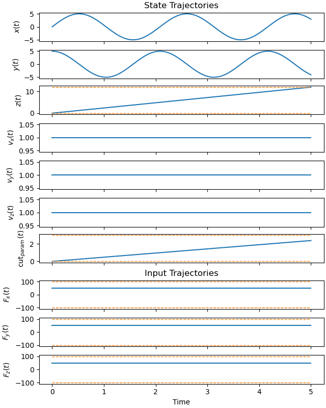
If a solution is available, it will be used as the initial guess.
fname = f'particle_in_tube_{num_nodes}_nodes_solution.csv'
if os.path.exists(fname):
initial_guess = np.loadtxt(fname)
par_map[faktor] = 0.25
solution, info = prob.solve(initial_guess)
print(info['status_msg'])
print(info['obj_val'])
b'Algorithm stopped at a point that was converged, not to "desired" tolerances, but to "acceptable" tolerances (see the acceptable-... options).'
39069.748698964104
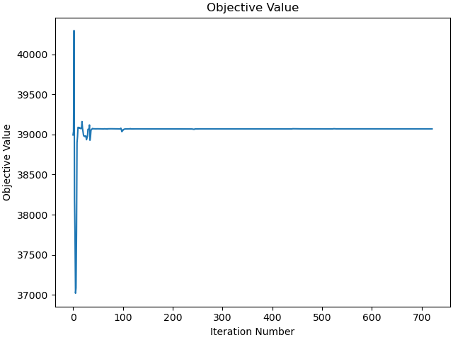
Plot the objective function as a function of optimizer iteration.
_ = prob.plot_objective_value()
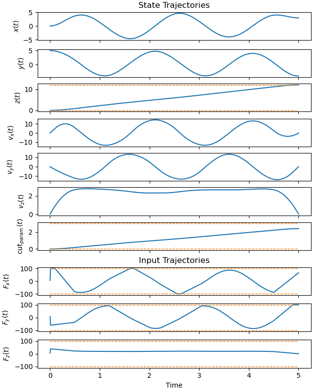
Plot the optimal state and input trajectories.
_ = prob.plot_trajectories(solution, show_bounds=True)
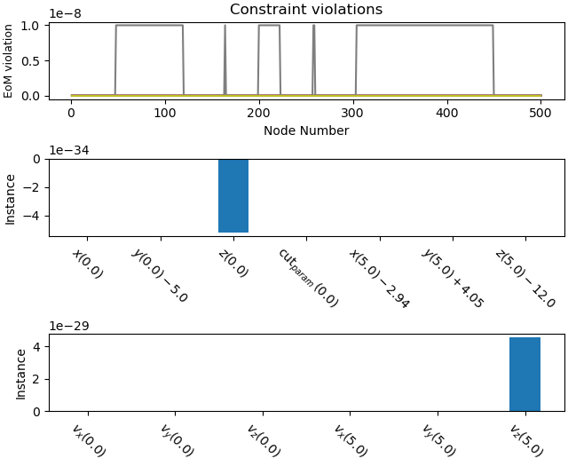
Plot the constraint violations.
_ = prob.plot_constraint_violations(solution)
Animate the Motion of the Particle
state_vals, input_vals, _ = prob.parse_free(solution)
t_arr = np.linspace(t0, duration, num_nodes)
state_sol = CubicSpline(t_arr, state_vals.T)
input_sol = CubicSpline(t_arr, input_vals.T)
fx, fy, fz = sm.symbols('fx, fy, fz', real=True)
Pf = me.Point('Pf')
Pf.set_pos(Dmc, fx*N.x + fy*N.y + fz*N.z)
time = np.linspace(0.0, duration, num=num_nodes)
coordinates = Dmc.pos_from(O).to_matrix(N)
coordinates = coordinates.row_join(Pf.pos_from(O).to_matrix(N))
eval_coords = sm.lambdify((state_symbols, fx, fy, fz, list(par_map.keys())),
coordinates, cse=True)
This function is to draw the tube which the particle must not leave.
def frenet_frame(f, g, h, r, num_points=100,
tube_radius=par_map[radius] + 0.25):
# Parameterize the curve
r_vals = r
f_vals = f(r_vals)
g_vals = g(r_vals)
h_vals = h(r_vals)
# Compute derivatives for tangent vectors
f_prime = np.gradient(f_vals, r_vals)
g_prime = np.gradient(g_vals, r_vals)
h_prime = np.gradient(h_vals, r_vals)
tangent_vectors = np.stack([f_prime, g_prime, h_prime], axis=-1)
tangent_vectors /= np.linalg.norm(tangent_vectors, axis=1)[:, np.newaxis]
# Approximate normal and binormal
normal_vectors = np.cross(tangent_vectors, np.roll(tangent_vectors, 1,
axis=0))
normal_vectors /= np.linalg.norm(normal_vectors, axis=1)[:, np.newaxis]
binormal_vectors = np.cross(tangent_vectors, normal_vectors)
# Create the circular cross-section
theta = np.linspace(0, 2 * np.pi, 30)
circle = np.stack([np.cos(theta), np.sin(theta)], axis=-1)
# Generate tube surface
X, Y, Z = [], [], []
for i in range(num_points):
frame = np.stack([normal_vectors[i], binormal_vectors[i]], axis=-1)
offset = circle @ frame.T * tube_radius
X.append(f_vals[i] + offset[:, 0])
Y.append(g_vals[i] + offset[:, 1])
Z.append(h_vals[i] + offset[:, 2])
return np.array(X), np.array(Y), np.array(Z)
This function draws a circle.
def plot_3d_circle(ax, center, radius, normal, num_points=100):
"""Plots a 3D circle based on the given center, radius, and normal vector.
Parameters
==========
center : ndarray
The center of the circle (numpy array of shape (3,))
radius : float
The radius of the circle (scalar)
normal : ndarray
The normal vector perpendicular to the circle's plane (numpy array of
shape (3,))
num_points : integer
The number of points used to plot the circle (default is 100)
"""
# Generate points on a circle in the xy-plane (z=0)
theta = np.linspace(0, 2 * np.pi, num_points)
x = radius * np.cos(theta)
y = radius * np.sin(theta)
z = np.zeros_like(theta)
# Create the points in the plane of the circle
circle_points = np.array([x, y, z])
# Normalize the normal vector to get the orientation of the circle plane
normal = normal / np.linalg.norm(normal)
# Find two perpendicular vectors to the normal
# (to define the plane of the circle)
# One of them can be chosen arbitrarily as long as it's not parallel
# to the normal
v1 = np.array([1, 2, 3]) / np.sqrt(1**2 + 2**2 + 3**2)
v1 = np.cross(normal, v1)
v1 = v1 / np.sqrt(np.sum([v1[i]**2 for i in range(3)]))
# Find the second perpendicular vector by crossing the normal and v1
v2 = np.cross(normal, v1)
# Parametrize the circle using v1 and v2 and translate to the center
circle_3d = (center[:, np.newaxis] +
v1[:, np.newaxis]*circle_points[0, :] +
v2[:, np.newaxis]*circle_points[1, :])
# Plot the 3D circle
ax.plot(circle_3d[0, :], circle_3d[1, :], circle_3d[2, :], color='blue')
class Vector3D(FancyArrowPatch):
"""Vector that can be animated in 3D."""
def __init__(self, xyz_tail, xyz_vec, *args, **kwargs):
super().__init__((0, 0), (0, 0), *args, **kwargs)
self._xyz_tail = xyz_tail
self._xyz_vec = xyz_vec
def do_3d_projection(self, renderer=None):
xs, ys, zs = proj_transform(
(self._xyz_tail[0], self._xyz_tail[0] + self._xyz_vec[0]),
(self._xyz_tail[1], self._xyz_tail[1] + self._xyz_vec[1]),
(self._xyz_tail[2], self._xyz_tail[2] + self._xyz_vec[2]),
self.axes.M)
self.set_positions((xs[0], ys[0]), (xs[1], ys[1]))
return min(zs)
def set_data(self, xyz_tail, xyz_vec):
self._xyz_tail = xyz_tail
self._xyz_vec = xyz_vec
Animate the motion of the particle. sphinx_gallery_thumbnail_number = 5
def init():
fig = plt.figure()
ax = fig.add_subplot(projection='3d')
arrow = Vector3D([0., 0., 0.], [1., 1., 1.], color='green', linewidth=2,
mutation_scale=6)
ax.add_artist(arrow)
line1, = ax.plot([], [], [], marker='o', color='black', markersize=7)
line2, = ax.plot([], [], [], color='black', lw=1)
ax.set_xlim(-par_map[a1] - 1, par_map[a1] + 1)
ax.set_ylim(-par_map[a2] - 1, par_map[a2] + 1)
ax.set_zlim(0.0, bounds[z][1] + 1)
ax.set_xlabel(r'$x$ [m]')
ax.set_ylabel(r'$y$ [m]')
ax.set_zlabel(r'$z$ [m]')
return fig, ax, line1, line2, arrow
fig, ax, line1, line2, arrow = init()
f = lambda r: eval_curve(r, par_map[a1], par_map[a2], par_map[a3])[0]
g = lambda r: eval_curve(r, par_map[a1], par_map[a2], par_map[a3])[1]
h = lambda r: eval_curve(r, par_map[a1], par_map[a2], par_map[a3])[2]
curve_param = np.linspace(0, max_z/par_map[a3], 100)
X, Y, Z = frenet_frame(f, g, h, r=curve_param)
ax.plot_surface(X, Y, Z, rstride=1, cstride=1, color='grey', alpha=0.1,
edgecolor='red')
center = np.array(eval_curve(1.2, par_map[a1], par_map[a2], par_map[a3]))
curvedt = [curve[i].diff(r) for i in range(3)]
eval_curvedt = sm.lambdify((r, a1, a2, a3), curvedt, cse=True)
normal = np.array(eval_curvedt(1.2, par_map[a1], par_map[a2], par_map[a3]))
normal = normal / np.sqrt([np.sum(normal[i]**2) for i in range(3)])
plot_3d_circle(ax, center=center, radius=par_map[radius]/3.0, normal=normal)
def animate(i):
fx1 = input_sol(time[i])[0]
fy1 = input_sol(time[i])[1]
fz1 = input_sol(time[i])[2]
skale = 13.0
coords = eval_coords(state_sol(time[i]), fx1, fy1, fz1,
list(par_map.values()))
arrow.set_data(coords[:, 0], (coords[:, 1] - coords[:, 0])/skale)
line1.set_data_3d([coords[0, 0]], [coords[1, 0]], [coords[2, 0]])
koords = []
for k in range(i):
koords.append(eval_coords(state_sol(time[k]), fx1, fy1, fz1,
list(par_map.values())))
line2.set_data_3d([koords[k][0][0] for k in range(i)],
[koords[k][1][0] for k in range(i)],
[koords[k][2][0] for k in range(i)])
ax.set_title(
f'Running time = {time[i]:.2f} s. \n The small blue circle '
f'is the gate \n The green arrow is proportional to the force.'
)
frames = [i for i in range(num_nodes)]
frames = frames[::10] + [frames[-1]]
ani = animation.FuncAnimation(fig, animate, frames,
interval=int(interval_value*10000))