Crane Moving a Load

Objectives

• Show the use of opty’s variable node time interval feature to solve a relatively simple problem.

• Show how to use additional specifieds to enforce instance constraints on \(\dfrac{d^2}{dt^2}(\textrm{state variable})\)

Introduction

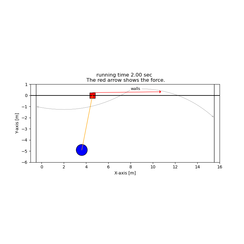
A load is moved by a crane. The load is connected to the crane by a massless rod and a pin joint. The goal is to move the load from the initial position to the final position in the shortest possible time. The load must not over-swing the final position. The load is moved by a force applied to its suspension point. The jib of the crane is extended in the horizontal X direction.

In order to ensure that the load is at rest at its final location, its velocity and its acceleration must be zero at the final time.

Notes

The solution opty finds may not what one would expect intuitively.

Constants

• \(l\) : length of the rod attaching the load to the crane [m]

• \(m_1\) : mass of mover attached to the arm of the crane [kg]

• \(m_2\) : mass of the load [kg]

• \(g\) : acceleration due to gravity [m/s²]

States

• \(x_c\) : x-coordinate of the mover [m]

• \(x_l\) : x-coordinate of the load [m]

• \(y_l\) : y-coordinate of the load [m]

• \(q\) : angle of the rod [rad]

• \(u_{xc}\) : velocity of the mover in x-direction [m/s]

• \(u_{xl}\) : velocity of the load in x-direction [m/s]

• \(u_{yl}\) : velocity of the load in y-direction [m/s]

• \(u\) : angular velocity of the rod [rad/s]

Specifieds

• \(F\) : force applied to the mover [N]

• \(h_1\) : needed to enforce instance constraints

• \(h_2\) : needed to enforce instance constraints

import os
import sympy.physics.mechanics as me
import numpy as np
import sympy as sm
from scipy.interpolate import CubicSpline
from opty.direct_collocation import Problem
from opty.utils import MathJaxRepr
import matplotlib.pyplot as plt
import matplotlib.animation as animation
from matplotlib import patches

Set up Kane’s Equations of Motion

N, A = sm.symbols('N A', cls=me.ReferenceFrame)
t = me.dynamicsymbols._t
O, P1, P2 = sm.symbols('O P1 P2', cls=me.Point)
O.set_vel(N, 0)
xc, xl, yl, q, uxc, uxl, uyl, u, F, h1, h2 = \
    me.dynamicsymbols('xc, xl, yl, q, uxc, uxl, uyl, uq, F, h1, h2')
l, m1, m2, g = sm.symbols('l, m1, m2, g')

A.orient_axis(N, q, N.z)
A.set_ang_vel(N, u*N.z)

P1.set_pos(O, xc*N.x)
P1.set_vel(N, uxc*N.x)

P2.set_pos(P1, -l*A.y)
P2.v2pt_theory(P1, N, A)

P1a = me.Particle('P1a', P1, m1)
P2a = me.Particle('P2a', P2, m2)

bodies = [P1a, P2a]

forces = [(P1, F*N.x - m1*g*N.y), (P2, -m2*g*N.y)]
kd = sm.Matrix([
    uxc - xc.diff(t),
    u - q.diff(t),
    uxl - xl.diff(t),
    uyl - yl.diff(t),
])

config_constr = sm.Matrix([xl - xc - l*sm.sin(q), yl + l*sm.cos(q)])
speed_constr = config_constr.diff(t)

q_ind = [xc, q]
q_dep = [xl, yl]
u_ind = [uxc, u]
u_dep = [uxl, uyl]

KM = me.KanesMethod(
    N,
    q_ind=q_ind,
    q_dependent=q_dep,
    u_ind=u_ind,
    u_dependent=u_dep,
    kd_eqs=kd,
    configuration_constraints=config_constr,
    velocity_constraints=speed_constr,
)

fr, frstar = KM.kanes_equations(bodies, forces)
eom = kd.col_join(fr + frstar)
eom = eom.col_join(config_constr)
eom = eom.col_join(sm.Matrix([h1 - u.diff(t),  h2 - uxc.diff(t)]))
MathJaxRepr(eom)

$$\left[\begin{matrix}uxc - \dot{xc}\\uq - \dot{q}\\uxl - \dot{xl}\\uyl - \dot{yl}\\l m_{2} uq^{2} \sin{\left(q \right)} - l m_{2} \cos{\left(q \right)} \dot{uq} - \left(m_{1} + m_{2}\right) \dot{uxc} + F\\- g l m_{2} \sin{\left(q \right)} - l^{2} m_{2} \dot{uq} - l m_{2} \cos{\left(q \right)} \dot{uxc}\\- l \sin{\left(q \right)} - xc + xl\\l \cos{\left(q \right)} + yl\\h_{1} - \dot{uq}\\h_{2} - \dot{uxc}\end{matrix}\right]$$

Set up the Optimization Problem and Solve it

state_symbols = tuple((*q_ind, *q_dep, *u_ind, *u_dep))
constant_symbols = (l, m1, m2, g)
specified_symbols = (F, h1, h2)
h = sm.symbols('h')

num_nodes = 150
duration = (num_nodes - 1)*h
interval_value = h

Specify the known system parameters.

par_map = {}
par_map[l] = 5.0
par_map[m1] = 1.0
par_map[m2] = 10.0
par_map[g] = 9.81

t0, tf = 0.0, duration

Set up the objective function and its gradient.

def obj(free):
    """Minimize h, the time interval between nodes."""
    return free[-1]


def obj_grad(free):
    grad = np.zeros_like(free)
    grad[-1] = 1.0
    return grad

Starting and final location of the load.

starting_location = 0.0
ending_location = 15.0

Form the instance constraints.

instance_constraints = (
    xc.func(t0) - starting_location,
    xl.func(t0) - starting_location,
    yl.func(t0) + par_map[l],
    q.func(t0),
    uxc.func(t0),
    uxl.func(t0),
    uyl.func(t0),
    u.func(t0),
    xc.func(tf) - ending_location,
    xl.func(tf) - ending_location,
    yl.func(tf) + par_map[l],
    q.func(tf),
    uxc.func(tf),
    uxl.func(tf),
    uyl.func(tf),
    u.func(tf),
    h1.func(tf),
    h2.func(tf),
)

Forcing h > 0.0 sometimes avoids negative ‘solutions’.

bounds = {
    F: (-20., 20.),
    xl: (starting_location, ending_location),
    xc: (starting_location, ending_location),
    h: (0.0, 1.0),
}

Create the optimization problem.

prob = Problem(
    obj,
    obj_grad,
    eom,
    state_symbols,
    num_nodes,
    interval_value,
    known_parameter_map=par_map,
    instance_constraints=instance_constraints,
    time_symbol=t,
    bounds=bounds,
    backend='numpy',
)

Reasonable initial guess.

i1 = [(ending_location - starting_location)/num_nodes*i for i in
      range(num_nodes)]
i2 = [0.0 for _ in range(num_nodes)]
i3 = i1
i4 = [-par_map[l] for _ in range(num_nodes)]
i5 = [0.0 for _ in range(5*num_nodes)]
i6 = list(np.zeros(2*num_nodes))
i7 = [0.01]
initial_guess = np.array(i1 + i2 + i3 + i4 + i5 + i6 + i7)

Use the the initial_guess given above and plot it.

_ = prob.plot_trajectories(initial_guess)

Use the solution of a previous run if available, else the initial guess given above is used to solve the problem.

fname = f'crane_moving_a_load_{num_nodes}_nodes_solution.csv'
if os.path.exists(fname):
    initial_guess = np.loadtxt(fname)

Find the optimal solution.

solution, info = prob.solve(initial_guess)
print('Message from optimizer:', info['status_msg'])
_ = prob.plot_objective_value()
print('Iterations needed', len(prob.obj_value))
print(f"Objective value {solution[-1]: .3e}")

Message from optimizer: b'Algorithm terminated successfully at a locally optimal point, satisfying the convergence tolerances (can be specified by options).'
Iterations needed 205
Objective value  3.956e-02

Plot the accuracy of the solution.

_ = prob.plot_constraint_violations(solution)

Plot the state trajectories.

_ = prob.plot_trajectories(solution, show_bounds=True)

Animate the Simulation

fps = 10

state_vals, input_vals, _, h_sol = prob.parse_free(solution)

tf = h_sol*(num_nodes - 1)
t_arr = prob.time_vector(solution=solution)
state_sol = CubicSpline(t_arr, state_vals.T)
input_sol = CubicSpline(t_arr, input_vals.T)

coordinates = P1.pos_from(O).to_matrix(N)
coordinates = coordinates.row_join(P2.pos_from(O).to_matrix(N))

pl, pl_vals = zip(*par_map.items())
coords_lam = sm.lambdify((*state_symbols, *specified_symbols, *pl),
                         coordinates, cse=True)

width, height, radius = 0.5, 0.5, 0.5


def init_plot():
    xmin, xmax = starting_location - 1, ending_location + 1
    ymin, ymax = -par_map[l] - 1, 1

    fig, ax = plt.subplots(figsize=(8, 8))
    ax.set_xlim(xmin, xmax)
    ax.set_ylim(ymin, ymax)
    ax.set_aspect('equal')
    ax.set_xlabel('X-axis [m]')
    ax.set_ylabel('Y-axis [m]')

    ax.axhline(0., color='black', lw=1.5)
    ax.axvline(ending_location+radius, color='black', lw=1.0)
    ax.axvline(starting_location-radius, color='black', lw=1.0)
    ax.annotate('walls', xy=(ending_location+radius, -2),
                arrowprops=dict(arrowstyle='->',
                                connectionstyle='arc3, rad=-.2',
                                lw=0.25),
                xytext=(8, 0.5), fontsize=9)
    ax.annotate('', xy=(starting_location-radius, -1),
                arrowprops=dict(arrowstyle='->',
                                connectionstyle='arc3, rad=-.2',
                                lw=0.25),
                xytext=(8, 0.5))

    line1, = ax.plot([], [], color='orange', lw=1)
    pfeil = ax.quiver([], [], [], [], color='red', scale=55, width=0.002,
                      headwidth=8)
    recht = patches.Rectangle((-width/2, -height/2), width=width,
                              height=height, fill=True, color='red',
                              ec='black')
    ax.add_patch(recht)
    load = patches.Circle((0, -par_map[l]), radius=radius, fill=True,
                          color='blue', ec='black')
    ax.add_patch(load)

    return fig, ax, line1, recht, load, pfeil


def update(t):
    message = f'running time {t:0.2f} sec \n The red arrow shows the force.'
    ax.set_title(message, fontsize=12)

    coords = coords_lam(*state_sol(t), *input_sol(t), *pl_vals)

    line1.set_data([coords[0, 0], coords[0, 1]], [coords[1, 0], coords[1, 1]])
    recht.set_xy((coords[0, 0] - width/2., coords[1, 0] - height/2.))
    load.set_center((coords[0, 1], coords[1, 1]))
    pfeil.set_offsets([coords[0, 0], coords[1, 0]+0.25])
    pfeil.set_UVC(input_sol(t)[0], 0.25)
    return line1, recht, load, pfeil

A frame from the animation.

fig, ax, line1, recht, load, pfeil = init_plot()
_ = update(2.0)

fig, ax, line1, recht, load, pfeil = init_plot()
anim = animation.FuncAnimation(fig, update,
                               frames=np.arange(t0, tf, 1/fps),
                               interval=1/fps*1000)

plt.show()

Once Loop Reflect