Upright a Double Pendulum

Objectives

• Show the use of opty’s variable time interval feature to solve a relatively simple problem.

• Show the use of specifieds to enforce terminal constraints on \(\dfrac{d^2}{dt^2}(\textrm{state variables})\).

Introduction

A double pendulum is rotationally attached to a cart which can move along the horizontal X axis. The goal is to get the double pendulum to an upright position in the shortest time possible, given an upper limit on the absolute value of the force that can be applied to the cart. Gravity points in the negative Y direction. To ensure that it is at rest, not only the speeds, but also its accelerations are constrained to be zero at the end of the motion.

Notes

The upright double pendulum seems to be a very standard example in physics. One can find a lot about it in the internet.

Constants

• \(m_1\): mass of the cart [kg]

• \(m_2\): mass of the first pendulum [kg]

• \(m_3\): mass of the second pendulum [kg]

• \(l_x\): length of the first pendulum rods [m]

• \(i_{ZZ1}\): moment of inertia of the first pendulum about its end point [kg*m^2]

• \(i_{ZZ2}\): moment of inertia of the second pendulum about its end point [kg*m^2]

• \(g\): acceleration due to gravity [m/s^2]

States

• \(q_1\): position of the cart along the X axis [m]

• \(q_2\): angle of the first pendulum with respect to the vertical [rad]

• \(q_3\): angle of the second pendulum with respect to the first [rad]

• \(u_1\): speed of the cart along the X axis [m/s]

• \(u_2\): angular speed of the first pendulum [rad/s]

• \(u_3\): angular speed of the second pendulum [rad/s]

Specifieds

• \(F\): force applied to the cart [N]

• \(h_1, h_2, h_3\) : needed to enforce the constraints on the accelerations of at the end of the motion.

import os
import numpy as np
import sympy as sm
import sympy.physics.mechanics as me
from opty import Problem
from opty.utils import MathJaxRepr
import matplotlib.pyplot as plt
import matplotlib.animation as animation
from matplotlib import patches

Equations of Motion, Kane’s Method

N, A1, A2 = sm.symbols('N A1, A2', cls=me.ReferenceFrame)
t = me.dynamicsymbols._t
O, P1, P2, P3 = sm.symbols('O P1 P2 P3', cls=me.Point)
O.set_vel(N, 0)
q1, q2, q3, u1, u2, u3, F = me.dynamicsymbols('q1 q2 q3 u1 u2 u3 F')
h1, h2, h3 = me.dynamicsymbols('h1 h2 h3')
lx, m1, m2, m3, g, iZZ1, iZZ2 = sm.symbols('lx, m1, m2, m3 g, iZZ1, iZZ2')

A1.orient_axis(N, q2, N.z)
A1.set_ang_vel(N, u2 * N.z)
A2.orient_axis(N, q3, N.z)
A2.set_ang_vel(N, u3 * N.z)

P1.set_pos(O, q1 * N.x)
P2.set_pos(P1, lx * A1.x)
P2.v2pt_theory(P1, N, A1)

P3.set_pos(P2, lx * A2.x)
P3.v2pt_theory(P2, N, A2)

P1a = me.Particle('P1a', P1, m1)

I1 = me.inertia(A1, 0, 0, iZZ1)
P2a = me.RigidBody('P2a', P2, A1, m2, (I1, P2))

I2 = me.inertia(A2, 0, 0, iZZ2)
P3a = me.RigidBody('P3a', P3, A2, m3, (I2, P3))
bodies = [P1a, P2a, P3a]

loads = [(P1, F * N.x - m1*g*N.y), (P2, -m2*g*N.y), (P3, -m3*g*N.y)]
kd = sm.Matrix([q1.diff(t) - u1, q2.diff(t) - u2, q3.diff(t) - u3])

q_ind = [q1, q2, q3]
u_ind = [u1, u2, u3]

KM = me.KanesMethod(
    N,
    q_ind=q_ind,
    u_ind=u_ind,
    kd_eqs=kd
)
fr, frstar = KM.kanes_equations(bodies, loads=loads)
eom = kd.col_join(fr + frstar)

add the auxiliary eoms for h1, h2, h3, so \(\dfrac{d^2}{dt^2}q_i(\textrm{duration}) = 0\) can be enforced.

eom = eom.col_join(sm.Matrix([h1 - u1.diff(t), h2 - u2.diff(t),
                   h3 - u3.diff(t)]))
eom = sm.simplify(eom)
MathJaxRepr(eom)

$$\left[\begin{matrix}- u_{1} + \dot{q}_{1}\\- u_{2} + \dot{q}_{2}\\- u_{3} + \dot{q}_{3}\\lx m_{2} u_{2}^{2} \cos{\left(q_{2} \right)} + lx m_{3} u_{2}^{2} \cos{\left(q_{2} \right)} + lx m_{3} u_{3}^{2} \cos{\left(q_{3} \right)} + lx m_{3} \sin{\left(q_{3} \right)} \dot{u}_{3} + lx \left(m_{2} + m_{3}\right) \sin{\left(q_{2} \right)} \dot{u}_{2} - \left(m_{1} + m_{2} + m_{3}\right) \dot{u}_{1} + F\\- g lx m_{2} \cos{\left(q_{2} \right)} - g lx m_{3} \cos{\left(q_{2} \right)} - lx^{2} m_{3} u_{3}^{2} \sin{\left(q_{2} - q_{3} \right)} - lx^{2} m_{3} \cos{\left(q_{2} - q_{3} \right)} \dot{u}_{3} + lx \left(m_{2} + m_{3}\right) \sin{\left(q_{2} \right)} \dot{u}_{1} - \left(iZZ_{1} + lx^{2} m_{2} + lx^{2} m_{3}\right) \dot{u}_{2}\\- g lx m_{3} \cos{\left(q_{3} \right)} + lx^{2} m_{3} u_{2}^{2} \sin{\left(q_{2} - q_{3} \right)} - lx^{2} m_{3} \cos{\left(q_{2} - q_{3} \right)} \dot{u}_{2} + lx m_{3} \sin{\left(q_{3} \right)} \dot{u}_{1} - \left(iZZ_{2} + lx^{2} m_{3}\right) \dot{u}_{3}\\h_{1} - \dot{u}_{1}\\h_{2} - \dot{u}_{2}\\h_{3} - \dot{u}_{3}\end{matrix}\right]$$

Set Up the Optimization Problem and Solve It

Define various objects to be use in the optimization problem.

h = sm.symbols('h')

state_symbols = tuple((*q_ind, *u_ind))
constant_symbols = (lx, m1, m2, m3, g, iZZ1, iZZ2)
specified_symbols = (F,)

target_angle = np.pi/2.0
num_nodes = 300

duration = (num_nodes - 1) * h
interval_value = h

Specify the known system parameters.

par_map = {}
par_map[lx] = 2.0
par_map[m1] = 1.0
par_map[m2] = 1.0
par_map[m3] = 1.0
par_map[g] = 9.81
par_map[iZZ1] = 2.0
par_map[iZZ2] = 2.0


def obj(free):
    """Minimize h, the time interval between nodes."""
    return free[-1]


def obj_grad(free):
    grad = np.zeros_like(free)
    grad[-1] = 1.0
    return grad

Set the initial and final states to form the instance constraints.

instance_constraints = (
    q1.func(0.0),
    q2.func(0.0) + np.pi/2.0,
    q3.func(0.0) + np.pi/2.0,
    u1.func(0.0),
    u2.func(0.0),
    u3.func(0.0),
    q2.func(duration) - target_angle,
    q3.func(duration) - target_angle,
    u1.func(duration),
    u2.func(duration),
    u3.func(duration),
    h1.func(duration),
    h2.func(duration),
    h3.func(duration),
)

Bounding h > 0 helps avoid ‘solutions’ with h < 0.

bounds = {
    F: (-50.0, 50.0),
    q1: (-5.0, 5.0),
    h: (0.0, 1.0),
}

Create an optimization problem and solve it.

prob = Problem(
    obj,
    obj_grad,
    eom,
    state_symbols,
    num_nodes,
    interval_value,
    known_parameter_map=par_map,
    instance_constraints=instance_constraints,
    time_symbol=t,
    bounds=bounds,
    backend='numpy'
)

# Initial guess.
initial_guess = np.zeros(prob.num_free)
initial_guess[1*num_nodes:2*num_nodes] = np.linspace(-target_angle,
                                                     target_angle,
                                                     num=num_nodes)
initial_guess[2*num_nodes:3*num_nodes] = np.linspace(-target_angle,
                                                     target_angle,
                                                     num=num_nodes)
initial_guess[6*num_nodes:7*num_nodes] = 50.0*np.ones(num_nodes)
initial_guess[-1] = 0.01

Use stored solution if available, else use initial_guess as given above.

fname = f'double_pendulum_on_a_cart_{num_nodes}_nodes_solution.csv'
if os.path.exists(fname):
    initial_guess = np.loadtxt(fname)

Find the optimal solution as no stored solution available.

solution, info = prob.solve(initial_guess)
print('Message from optimizer:', info['status_msg'])
print('Iterations needed', len(prob.obj_value))
print(f"Objective value {solution[-1]: .3e}")

Message from optimizer: b'Algorithm terminated successfully at a locally optimal point, satisfying the convergence tolerances (can be specified by options).'
Iterations needed 68
Objective value  9.780e-03

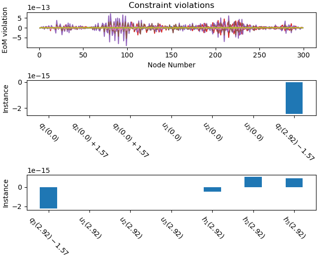
Plot the accuracy of the solution.

_ = prob.plot_constraint_violations(solution)

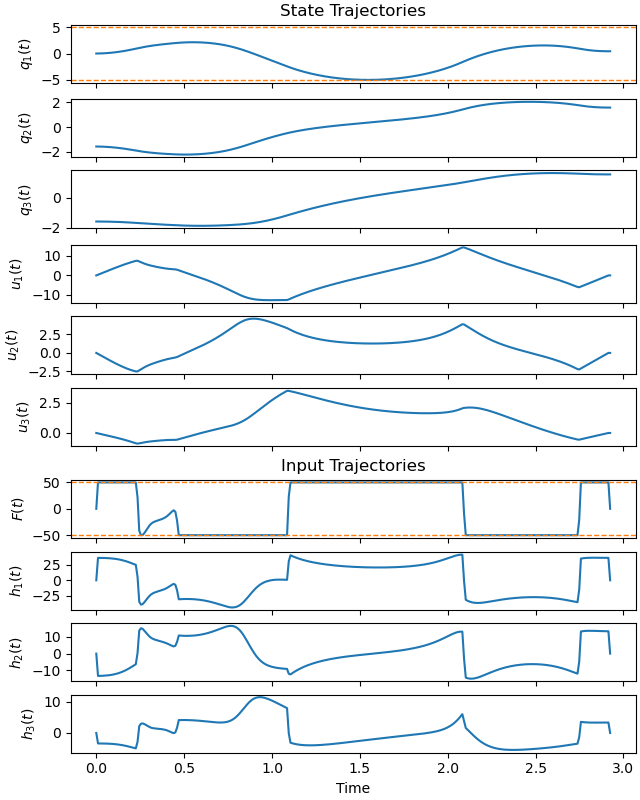
Plot the state trajectories.

_ = prob.plot_trajectories(solution, show_bounds=True)

Animate the Solution

state_sol, _, _, h_var = prob.parse_free(solution)
state_sol1 = state_sol.T[::4, :]
num_nodes = state_sol1.shape[0]
solution = list(state_sol1.T.flatten()) + [h_var]

P1_x = np.empty(num_nodes)
P1_y = np.empty(num_nodes)
P2_x = np.empty(num_nodes)
P2_y = np.empty(num_nodes)
P3_x = np.empty(num_nodes)
P3_y = np.empty(num_nodes)

P1_loc = [me.dot(P1.pos_from(O), uv) for uv in [N.x, N.y]]
P2_loc = [me.dot(P2.pos_from(O), uv) for uv in [N.x, N.y]]
P3_loc = [me.dot(P3.pos_from(O), uv) for uv in [N.x, N.y]]

qL = q_ind + u_ind
pL_vals = list(constant_symbols)
P1_loc_lam = sm.lambdify(qL + pL_vals, P1_loc, cse=True)
P2_loc_lam = sm.lambdify(qL + pL_vals, P2_loc, cse=True)
P3_loc_lam = sm.lambdify(qL + pL_vals, P3_loc, cse=True)

for i in range(num_nodes):
    q_1 = solution[i]
    q_2 = solution[i + num_nodes]
    q_3 = solution[i + 2 * num_nodes]
    u_1 = solution[i + 3 * num_nodes]
    u_2 = solution[i + 4 * num_nodes]
    u_3 = solution[i + 5 * num_nodes]
    P1_x[i], P1_y[i] = P1_loc_lam(q_1, q_2, q_3, u_1, u_2, u_3,
                                  *list(par_map.values()))
    P2_x[i], P2_y[i] = P2_loc_lam(q_1, q_2, q_3, u_1, u_2, u_3,
                                  *list(par_map.values()))
    P3_x[i], P3_y[i] = P3_loc_lam(q_1, q_2, q_3, u_1, u_2, u_3,
                                  *list(par_map.values()))


# needed to give the picture the right size.
xmin = min(np.min(P1_x), np.min(P2_x), np.min(P3_x))
xmax = max(np.max(P1_x), np.max(P2_x), np.max(P3_x))
ymin = min(np.min(P1_y), np.min(P2_y), np.min(P3_y))
ymax = max(np.max(P1_y), np.max(P2_y), np.max(P3_y))

width, height = par_map[lx]/3., par_map[lx]/3.


def animate_pendulum(time, P1_x, P1_y, P2_x, P2_y):

    fig, ax = plt.subplots(figsize=(8, 8), subplot_kw={'aspect': 'equal'})

    ax.axis('on')
    ax.set_xlim(xmin - 1., xmax + 1.)
    ax.set_ylim(ymin - 1., ymax + 1.)

    ax.set_xlabel('X direction', fontsize=15)
    ax.set_ylabel('Y direction', fontsize=15)
    ax.axhline(0, color='black', lw=2)

    line1, = ax.plot([], [], 'o-', lw=0.5, color='blue')
    line2, = ax.plot([], [], 'o-', lw=0.5, color='green')

    recht = patches.Rectangle((P1_x[0] - width/2, P1_y[0] - height/2),
                              width=width, height=height, fill=True,
                              color='red', ec='black')
    ax.add_patch(recht)
    return fig, ax, line1, line2, recht


duration = (num_nodes - 1) * solution[-1] * 4
times = np.linspace(0.0, duration, num_nodes)


def animate(i):
    message = (f'running time {times[i]: .2f} sec')
    ax.set_title(message, fontsize=15)
    recht.set_xy((P1_x[i] - width/2., P1_y[i] - height/2.))

    wert_x = [P1_x[i], P2_x[i]]
    wert_y = [P1_y[i], P2_y[i]]
    line1.set_data(wert_x, wert_y)

    wert_x = [P2_x[i], P3_x[i]]
    wert_y = [P2_y[i], P3_y[i]]
    line2.set_data(wert_x, wert_y)
    return line1, line2,

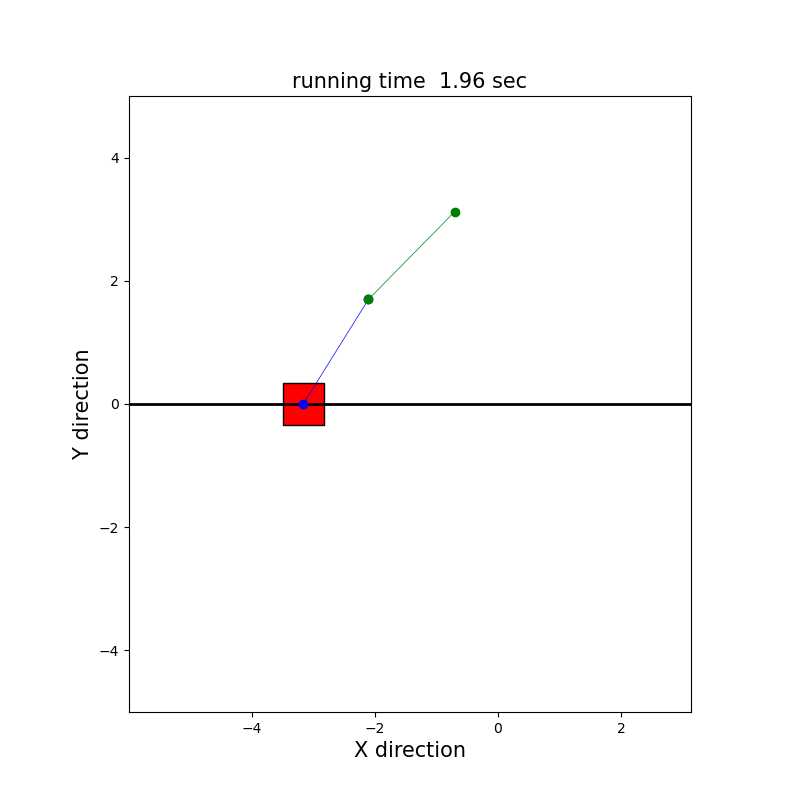
A frame from the animation.

fig, ax, line1, line2, recht = animate_pendulum(times, P1_x, P1_y, P2_x, P2_y)


_ = animate(50)

fig, ax, line1, line2, recht = animate_pendulum(times, P1_x, P1_y, P2_x, P2_y)
anim = animation.FuncAnimation(fig, animate, frames=num_nodes,
                               interval=solution[-1]*1000.0 * 4)

plt.show()

Once Loop Reflect