Bicycle Countersteering

Objectives

• Demonstrate using kinematic inputs (and their time derivatives) as the unknown input trajectories.

Introduction

The simplest model of a bicycle that exhibits countersteering can be created by adding a inverted pendulum atop the “bicycle model” of the car. [Bourlet1899] and others created early examples of this model, but we use the formulation from [Karnopp2004] here.

The goal of this optimal control problem is to find the steering control input to make a 90 degree right-hand turn in minimal time with limits on steer and roll angular rate while traveling at 18 km/h.

from opty import Problem
from opty.utils import MathJaxRepr
import matplotlib.pyplot as plt
import matplotlib.animation as animation
import numpy as np
import sympy as sm
import sympy.physics.mechanics as me

Specify the equations of motion

The model is constructed using several constant parameters:

• \(h\): distance mass center is from the ground contact line

• \(a\): longitudinal distance of the mass center from the rear contact

• \(b\): wheelbase length

• \(v\): constant longitudinal speed at the rear contact

• \(g\): acceleration due to gravity

• \(m\): mass of bicycle and rider

• \(I_1\): roll principle moment of inertia

• \(I_2\): pitch principle moment of inertia

• \(I_3\): yaw principle moment of inertia

h, a, b, v, g = sm.symbols('h a, b, v, g', real=True)
m, I1, I2, I3 = sm.symbols('m, I1, I2, I3', real=True)

The essential dynamics are described by a single degree of freedom model with roll angle \(\theta\) and its angular rate \(\omega=\dot{\theta}\) being the essential state variables. The location of the rear contact in the ground plane \(x,y\) and heading \(\psi\) will also be tracked. The input is the steering angle \(\delta\).

theta, omega = me.dynamicsymbols('theta, omega', real=True)
x, y, psi = me.dynamicsymbols('x, y, psi', real=True)
delta, beta = me.dynamicsymbols('delta, beta', real=True)
t = me.dynamicsymbols._t

The first two differential equations are the essential single degree of freedom dynamics followed by the differential equations to track \(x,y\) and \(\psi\). Both \(\delta\) and \(\beta=\dot{\delta}\) are present as inputs to the dynamics. In the optimal control problem, both of these input trajectories are sought with the constraint that \(\beta=\dot{\delta}\) holds. To manage this with opty, add a differential equation that ensures steering angle and steering rate variables are related by time differentiation and make \(\delta\) a pseudo state variable with the highest derivative \(\beta\) being the single unknown input trajectory.

eom = sm.Matrix([
    theta.diff(t) - omega,
    (I1 + m*h**2)*omega.diff(t) +
    (I3 - I2 - m*h**2)*(v*sm.tan(delta)/b)**2*sm.sin(theta)*sm.cos(theta) -
    m*g*h*sm.sin(theta) +
    m*h*sm.cos(theta)*(a*v/b/sm.cos(delta)**2*beta +
                       v**2/v*sm.tan(delta)),
    x.diff(t) - v*sm.cos(psi),
    y.diff(t) - v*sm.sin(psi),
    psi.diff(t) - v/b*sm.tan(delta),
    delta.diff(t) - beta,
])
MathJaxRepr(eom)

$$\left[\begin{matrix}- \omega + \dot{\theta}\\- g h m \sin{\left(\theta \right)} + h m \left(\frac{a v \beta}{b \cos^{2}{\left(\delta \right)}} + v \tan{\left(\delta \right)}\right) \cos{\left(\theta \right)} + \left(I_{1} + h^{2} m\right) \dot{\omega} + \frac{v^{2} \left(- I_{2} + I_{3} - h^{2} m\right) \sin{\left(\theta \right)} \cos{\left(\theta \right)} \tan^{2}{\left(\delta \right)}}{b^{2}}\\- v \cos{\left(\psi \right)} + \dot{x}\\- v \sin{\left(\psi \right)} + \dot{y}\\\dot{\psi} - \frac{v \tan{\left(\delta \right)}}{b}\\- \beta + \dot{\delta}\end{matrix}\right]$$

state_symbols = (theta, omega, x, y, psi, delta)
MathJaxRepr(state_symbols)

$$\left( \theta, \ \omega, \ x, \ y, \ \psi, \ \delta\right)$$

Provide some reasonably realistic values for the constants.

par_map = {
    I1: 9.2,  # kg m^2
    I2: 11.0,  # kg m^2
    I3: 2.8,  # kg m^2
    a: 0.5,  # m
    b: 1.0,  # m
    g: 9.81,  # m/s^2
    h: 1.0,  # m
    m: 87.0,  # kg
    v: 5.0,  # m/s
}

Define the optimal control problem

Instance constraints can be set on any of the state variables. The goal is to transition from cruising at a steady state in balance equilibrium to steady state in balance equilibrium with a 90 degree change in heading, i.e. make a right turn.

num_nodes = 201
dt = sm.symbols('Delta_t', real=True)
start = 0*dt
end = (num_nodes - 1)*dt

instance_constraints = (
    # upright, no motion at t = start
    theta.func(0*dt),
    omega.func(0*dt),
    x.func(0*dt),
    y.func(0*dt),
    psi.func(0*dt),
    delta.func(0*dt),
    # upright, no motion, 90 deg heading at t = end
    theta.func(end),
    omega.func(end),
    psi.func(end) - np.deg2rad(90.0),
    delta.func(end),
)

Specify the objective function and its gradient. Minimize the time required to go from the start state to the end state.

def objective(free):
    """Return h (always the last element in the free variables)."""
    return free[-1]


def gradient(free):
    """Return the gradient of the objective."""
    grad = np.zeros_like(free)
    grad[-1] = 1.0
    return grad

Add some physical limits to the states and inputs. Given that the steering is massless in this model, the solution will be governed by how fast the model can move. The limits on steer angular rate and roll angular rate will dictate the form of solution.

bounds = {
    psi: (np.deg2rad(-360.0), np.deg2rad(360.0)),
    theta: (np.deg2rad(-90.0), np.deg2rad(90.0)),
    delta: (np.deg2rad(-90.0), np.deg2rad(90.0)),
    beta: (np.deg2rad(-200.0), np.deg2rad(200.0)),
    omega: (np.deg2rad(-100.0), np.deg2rad(100.0)),
    dt: (0.001, 0.5),
}

Create the optimization problem and set any options.

prob = Problem(objective, gradient, eom, state_symbols, num_nodes, dt,
               known_parameter_map=par_map,
               instance_constraints=instance_constraints, bounds=bounds,
               time_symbol=t, backend='numpy')

Solve the optimal control problem

Make a simple initial guess.

initial_guess = 0.01*np.ones(prob.num_free)

Find the optimal solution.

solution, info = prob.solve(initial_guess)

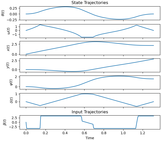
Plot the optimal state and input trajectories.

_ = prob.plot_trajectories(solution)

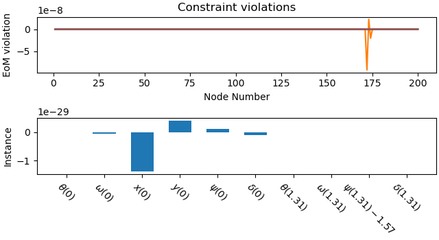
Plot the constraint violations.

_ = prob.plot_constraint_violations(solution)

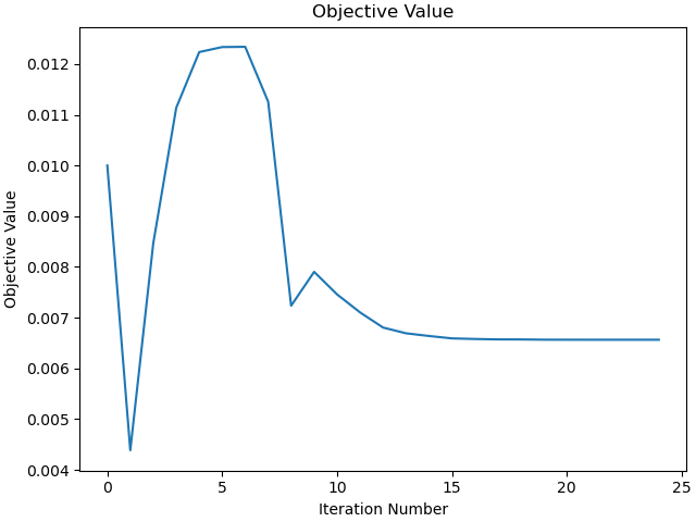
Plot the objective function as a function of optimizer iteration.

_ = prob.plot_objective_value()

Animate the motion

xs, us, ps, dt_val = prob.parse_free(solution)


def bicycle_points(x):
    """Return x, y, z coordinates of points that draw the bicycle model.

    Parameters
    ==========
    x : array_like, shape(n, N)
        n state trajectories over N time steps.

    Returns
    =======
    coordinates : ndarray, shape(N, 7, 3)
        Coordinates of the seven points over time.

    """
    coordinates = np.empty((x.shape[1], 7, 3))

    for i, xi in enumerate(x.T):

        theta, omega, x, y, psi, delta = xi

        rear_contact = np.array([x, y, 0.0])
        com_on_ground = rear_contact + np.array([par_map[a]*np.cos(psi),
                                                 par_map[a]*np.sin(psi),
                                                 0.0])
        com = com_on_ground + np.array([-par_map[h]*np.sin(theta)*np.sin(psi),
                                        par_map[h]*np.sin(theta)*np.cos(psi),
                                        -par_map[h]*np.cos(theta)])
        front_contact = rear_contact + np.array([par_map[b]*np.cos(psi),
                                                 par_map[b]*np.sin(psi),
                                                 0.0])
        front_steer = front_contact + np.array([0.2*np.cos(delta + psi),
                                                0.2*np.sin(delta + psi),
                                                0.0])
        rear_steer = front_contact + np.array([-0.2*np.cos(delta + psi),
                                               -0.2*np.sin(delta + psi),
                                               0.0])
        coordinates[i] = np.vstack((rear_contact, com_on_ground, com,
                                    com_on_ground, front_contact, front_steer,
                                    rear_steer))
    return coordinates


coordinates = bicycle_points(xs)

def frame(i):

    fig = plt.figure()
    ax = fig.add_subplot(projection='3d')

    x, y, z = coordinates[i].T

    bike_lines, = ax.plot(x, y, z, color='black', marker='o',
                          markerfacecolor='C0', markersize=4)
    rear_path, = ax.plot(coordinates[:i, 0, 0],
                         coordinates[:i, 0, 1],
                         coordinates[:i, 0, 2], color='C1')
    front_path, = ax.plot(coordinates[:i, 4, 0],
                          coordinates[:i, 4, 1],
                          coordinates[:i, 4, 2], color='C2')

    ax.yaxis.set_inverted(True)
    ax.zaxis.set_inverted(True)
    ax.set_xlim((0.0, 4.0))
    ax.set_ylim((3.0, -1.0))
    ax.set_zlim((0.0, -4.0))
    ax.set_xlabel(r'$x$ [m]')
    ax.set_ylabel(r'$y$ [m]')
    ax.set_zlabel(r'$z$ [m]')

    return fig, bike_lines, rear_path, front_path


fig, bike_lines, rear_path, front_path = frame(0)


def animate(i):
    x, y, z = coordinates[i].T
    bike_lines.set_data_3d(x, y, z)
    rear_path.set_data_3d(coordinates[:i, 0, 0],
                          coordinates[:i, 0, 1],
                          coordinates[:i, 0, 2])
    front_path.set_data_3d(coordinates[:i, 4, 0],
                           coordinates[:i, 4, 1],
                           coordinates[:i, 4, 2])


ani = animation.FuncAnimation(fig, animate, num_nodes,
                              interval=int(dt_val*1000))

plt.show()

Once Loop Reflect