Note
Go to the end to download the full example code.
Parallel Park a Car
Given the nonholonomic bicycle model of the car find a solution for parallel parking it.
Constants
m : car mass, [kg]
I : car yaw moment of inertia, [kg m^2]
a : distance from front axle to mass center, [m]
b : distance from rear axle to mass center, [m]
States
x : position of mass center, [m]
y : position of mass center, [m]
theta : yaw angle of the car, [rad]
delta : steer angle of the front wheels relative to the car, [rad]
vx : longitudinal speed of the car’s mass center, [m/s]
vy : lateral speed of the car’s mass center, [m/s]
omega : yaw angular rate of the car, [rad/s]
beta : steer angular rate of the front wheels relative to the car, [rad/s]
Specifieds
F : longitudinal propulsion force, [N]
T : steering torque, [N m]
import numpy as np
import sympy as sm
import sympy.physics.mechanics as me
from opty import Problem, create_objective_function
import matplotlib.pyplot as plt
import matplotlib.animation as animation
Generate the nonholonomic equations of motion of the system.
m, I, a, b = sm.symbols('m, I, a, b', real=True)
x, y, vx, vy = me.dynamicsymbols('x, y, v_x, v_y', real=True)
theta, omega = me.dynamicsymbols('theta, omega', real=True)
delta, beta = me.dynamicsymbols('delta, beta', real=True)
T, F = me.dynamicsymbols('T, F', real=True)
t = me.dynamicsymbols._t
O, Ao, Pr, Pf = sm.symbols('O, A_o, P_r, P_F', cls=me.Point)
N, A, B = sm.symbols('N, A, B', cls=me.ReferenceFrame)
A.orient_axis(N, theta, N.z)
B.orient_axis(A, delta, A.z)
Ao.set_pos(O, x*N.x + y*N.y)
Pr.set_pos(Ao, -b*A.x)
Pf.set_pos(Ao, a*A.x)
A.set_ang_vel(N, omega*N.z)
kinematical = [
vx - (x.diff()*N.x + y.diff()*N.y).dot(A.x),
vy - (x.diff()*N.x + y.diff()*N.y).dot(A.y),
omega - theta.diff(),
beta - delta.diff(),
]
O.set_vel(N, 0)
Ao.set_vel(N, vx*A.x + vy*A.y)
Pr.v2pt_theory(Ao, N, A)
Pf.v2pt_theory(Ao, N, A)
nonholonomic = [
Pr.vel(N).dot(A.y),
Pf.vel(N).dot(B.y),
]
IA = me.inertia(A, 0, 0, I)
car = me.RigidBody('A', Ao, A, m, (IA, Ao))
IB = me.inertia(B, 0, 0, I/32)
wheel = me.RigidBody('B', Pf, B, m/6, (IB, Pf))
propulsion = (Pr, F*A.x)
steeringA = (A, -T*B.z)
steeringB = (B, T*B.z)
kane = me.KanesMethod(
N,
[x, y, theta, delta],
[vx, beta],
kd_eqs=kinematical,
u_dependent=[vy, omega],
velocity_constraints=nonholonomic,
)
fr, frstar = kane.kanes_equations([car, wheel],
[propulsion, steeringA, steeringB])
eom = (fr + frstar).col_join(
sm.Matrix(nonholonomic)).col_join(
sm.Matrix(kinematical))
sm.pprint(eom)
⎡ ⎛ d d ⎞ ↪
⎢ ⎜ a⋅m⋅──(ω(t)) 7⋅m⋅──(v_y(t))⎟ ↪
⎢ ⎜ dt 7⋅m⋅ω(t)⋅vₓ(t) dt ⎟ ↪
⎢b⋅⎜- ──────────── - ────────────── - ──────────────⎟⋅sin(δ(t)) ↪
⎢ ⎝ 6 6 6 ⎠ m⋅(a⋅ω(t) + ↪
⎢────────────────────────────────────────────────────────────── + ──────────── ↪
⎢ a⋅cos(δ(t)) + b⋅cos(δ(t)) 6 ↪
⎢ ↪
⎢ ↪
⎢ ↪
⎢ ↪
⎢ ↪
⎢ ↪
⎢ ↪
⎢ ↪
⎢ ↪
⎢ ↪
⎢ ↪
⎢ ↪
⎢ ↪
⎢ ↪
⎢ ↪
⎢ ↪
⎢ ↪
⎢ ↪
⎢ ↪
⎢ ↪
⎢ ↪
⎢ ↪
⎢ ↪
⎢ ↪
⎢ ↪
⎣ ↪
↪ ⎛ d ↪
↪ ⎜ I⋅──(β(t)) ↪
↪ d ⎜ dt a⋅m⋅ω( ↪
↪ 7⋅m⋅──(vₓ(t)) ⎜- ────────── - ────── ↪
↪ v_y(t))⋅ω(t) dt ⎝ 32 ↪
↪ ──────────── + m⋅ω(t)⋅v_y(t) - ───────────── + F(t) + ────────────────────── ↪
↪ 6 ↪
↪ ↪
↪ d d ↪
↪ I⋅──(β(t)) I⋅──(ω(t)) ↪
↪ dt dt ↪
↪ - ────────── - ────────── + T(t) ↪
↪ 32 32 ↪
↪ ↪
↪ -b⋅ω(t) + v_y(t) ↪
↪ ↪
↪ (a⋅ω(t) + v_y(t))⋅cos(δ(t)) - vₓ(t)⋅sin(δ(t)) ↪
↪ ↪
↪ d d ↪
↪ vₓ(t) - sin(θ(t))⋅──(y(t)) - cos(θ(t))⋅──(x(t)) ↪
↪ dt dt ↪
↪ ↪
↪ d d ↪
↪ v_y(t) + sin(θ(t))⋅──(x(t)) - cos(θ(t))⋅──(y(t)) ↪
↪ dt dt ↪
↪ ↪
↪ d ↪
↪ ω(t) - ──(θ(t)) ↪
↪ dt ↪
↪ ↪
↪ d ↪
↪ β(t) - ──(δ(t)) ↪
↪ dt ↪
↪ d ⎞ ⎤
↪ a⋅m⋅──(v_y(t)) ⎛ 2 ⎞ ⎟ ⎥
↪ t)⋅vₓ(t) dt ⎜33⋅I a ⋅m⎟ d ⎟ ⎥
↪ ──────── - ────────────── - ⎜──── + ────⎟⋅──(ω(t))⎟⋅sin(δ(t))⎥
↪ 6 6 ⎝ 32 6 ⎠ dt ⎠ ⎥
↪ ─────────────────────────────────────────────────────────────⎥
↪ a⋅cos(δ(t)) + b⋅cos(δ(t)) ⎥
↪ ⎥
↪ ⎥
↪ ⎥
↪ ⎥
↪ ⎥
↪ ⎥
↪ ⎥
↪ ⎥
↪ ⎥
↪ ⎥
↪ ⎥
↪ ⎥
↪ ⎥
↪ ⎥
↪ ⎥
↪ ⎥
↪ ⎥
↪ ⎥
↪ ⎥
↪ ⎥
↪ ⎥
↪ ⎥
↪ ⎥
↪ ⎥
↪ ⎥
↪ ⎦
Set up the time discretization.
duration = 30.0 # seconds
num_nodes = 501
interval_value = duration/(num_nodes - 1)
Provide some reasonably realistic values for the constants.
par_map = {
I: 1/12*1200*(2**2 + 3**2),
m: 1200,
a: 1.5,
b: 1.5,
}
state_symbols = (x, y, theta, delta, vx, vy, omega, beta)
specified_symbols = (T, F)
Specify the objective function and form the gradient.
obj_func = sm.Integral(F**2 + T**2, t)
sm.pprint(obj_func)
obj, obj_grad = create_objective_function(obj_func,
state_symbols,
specified_symbols,
tuple(),
num_nodes,
interval_value,
time_symbol=t)
⌠
⎮ ⎛ 2 2 ⎞
⎮ ⎝F (t) + T (t)⎠ dt
⌡
Specify the symbolic instance constraints, i.e. initial and end conditions. The car should be stationary at start and stop but laterally displaced 2 meters (car width).
instance_constraints = (
x.func(0.0),
y.func(0.0),
theta.func(0.0),
delta.func(0.0),
vx.func(0.0),
vy.func(0.0),
omega.func(0.0),
beta.func(0.0),
x.func(duration),
y.func(duration) - 2.0,
theta.func(duration),
delta.func(duration),
vx.func(duration),
vy.func(duration),
omega.func(duration),
beta.func(duration),
)
Add some physical limits to some variables.
bounds = {
delta: (np.deg2rad(-45.0), np.deg2rad(45.0)),
T: (-50.0, 50.0),
F: (-300.0, 300.0),
}
Create the optimization problem and set any options.
prob = Problem(obj, obj_grad, eom, state_symbols,
num_nodes, interval_value,
known_parameter_map=par_map,
instance_constraints=instance_constraints,
bounds=bounds, time_symbol=t)
prob.add_option('nlp_scaling_method', 'gradient-based')
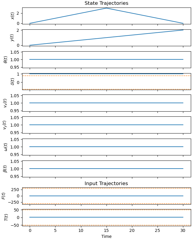
Give some rough estimates for the x and y trajectories.
time = prob.time_vector()
x_guess = 3.0/duration*2.0*time
x_guess[num_nodes//2:] = 6.0 - 3.0/duration*2.0*time[num_nodes//2:]
y_guess = 2.0/duration*time
initial_guess = np.ones(prob.num_free)
initial_guess[:num_nodes] = x_guess
initial_guess[num_nodes:2*num_nodes] = y_guess
_ = prob.plot_trajectories(initial_guess, show_bounds=True)
Find the optimal solution.
solution, info = prob.solve(initial_guess)
print(info['status_msg'])
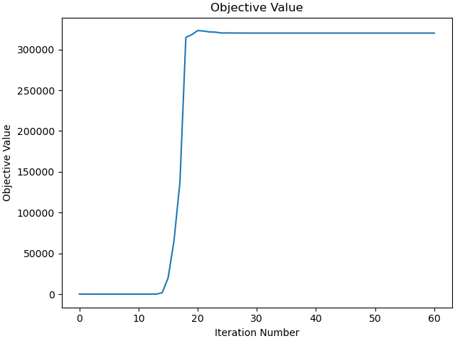
print(info['obj_val'])
b'Algorithm terminated successfully at a locally optimal point, satisfying the convergence tolerances (can be specified by options).'
320112.3735945718
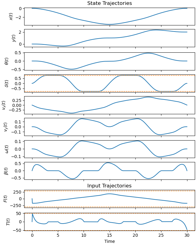
Plot the optimal state and input trajectories.
_ = prob.plot_trajectories(solution, show_bounds=True)
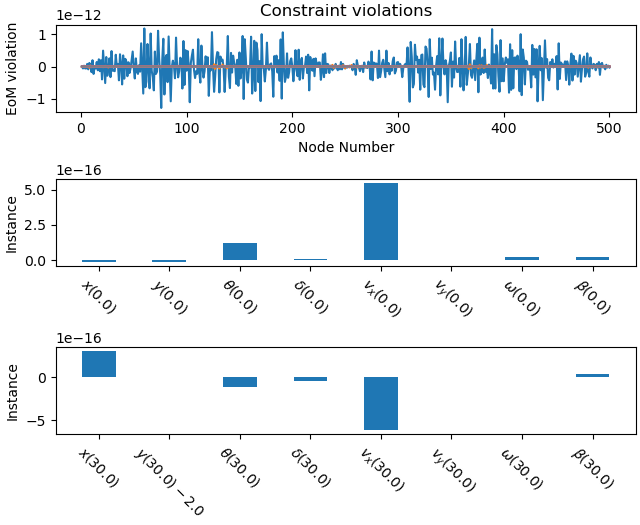
Plot the constraint violations.
_ = prob.plot_constraint_violations(solution)
Plot the objective function as a function of optimizer iteration.
_ = prob.plot_objective_value()
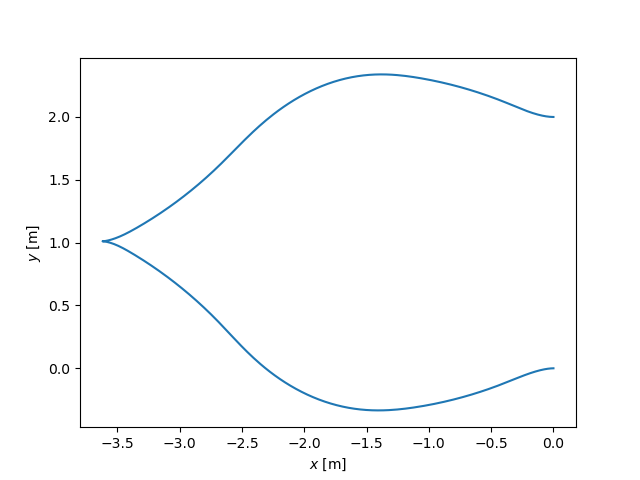
Show the optimal path of the mass center.
xs, us, ps = prob.parse_free(solution)
fig, ax = plt.subplots()
ax.plot(xs[0], xs[1])
ax.set_xlabel(r'$x$ [m]')
ax.set_ylabel(r'$y$ [m]');
Text(42.597222222222214, 0.5, '$y$ [m]')
Animate the motion of the car.
points = [Ao, Pf, Pf.locatenew('Bf', a/4*B.x), Pf.locatenew('Br', -a/4*B.x)]
coordinates = Pr.pos_from(O).to_matrix(N)
for point in points:
coordinates = coordinates.row_join(point.pos_from(O).to_matrix(N))
eval_point_coords = sm.lambdify((state_symbols, specified_symbols,
list(par_map.keys())), coordinates)
coords = []
for xi, ui in zip(xs.T, us.T):
coords.append(eval_point_coords(xi, ui, list(par_map.values())))
coords = np.array(coords) # shape(600, 3, 8)
def frame(i):
fig, ax = plt.subplots()
ax.set_aspect('equal')
x, y, z = eval_point_coords(xs[:, i], us[:, i], list(par_map.values()))
lines, = ax.plot(x, y, color='black', marker='o', markerfacecolor='blue',
markersize=4)
Pr_path, = ax.plot(coords[:i, 0, 0], coords[:i, 1, 0])
Pf_path, = ax.plot(coords[:i, 0, 2], coords[:i, 1, 2])
title_template = 'Time = {:1.2f} s'
title_text = ax.set_title(title_template.format(time[i]))
ax.set_xlim((np.min(coords[:, 0, :]) - 0.2,
np.max(coords[:, 0, :]) + 0.2))
ax.set_ylim((np.min(coords[:, 1, :]) - 0.2,
np.max(coords[:, 1, :]) + 0.2))
ax.set_xlabel(r'$x$ [m]')
ax.set_ylabel(r'$y$ [m]')
return fig, title_text, lines, Pr_path, Pf_path
fig, title_text, lines, Pr_path, Pf_path = frame(0)
def animate(i):
title_text.set_text('Time = {:1.2f} s'.format(time[i]))
lines.set_data(coords[i, 0, :], coords[i, 1, :])
Pr_path.set_data(coords[:i, 0, 0], coords[:i, 1, 0])
Pf_path.set_data(coords[:i, 0, 2], coords[:i, 1, 2])
ani = animation.FuncAnimation(fig, animate, len(time),
interval=int(interval_value*1000))