Note
Go to the end to download the full example code.
Quarter Car Model on a Bumpy Road
Objectives
Show on a simple example how to simultaneously optimize free parameters and unknown trajectories of a system.
Show how to use an unknown input trajectory to get the acceleration of a body into the objective function.
Show how to use bounds on the equations of motion.
Show how to avoid possible unwanted unknown trajectories (here \(\dfrac{d^2}{dt^2}x_{car}\)).
Introduction
A quarter car model must move from a starting point to a final point on a bumpy road. The body (sprung mass) is connected to the wheel (unsprung mass) on the road by a linear spring and a damper. Body and wheel are modeled by particles. Movement is in the X/Z plane. Gravity points in the negative Z direction.
The tire stiffness was taken from here:
https://kktse.github.io/jekyll/update/2021/07/18/re71r-255-40-r17-tire-vertical-stiffness.html
The goal is to minimize the acceleration of the body, given the road and the optimum driving force, by selecting the optimal values of the spring constant, and of the damping constant. The driving force must get the quarter wheel car from its starting point to its final point, while minimizing the objective function.
States
\(x_{\textrm{car}}\) : x position of the car [m]
\(z_{\textrm{car}}\) : z position of the car [m]
\(z_{\textrm{wheel}}\) : z position of the wheel [m]
\(ux_{\textrm{car}}\) : x velocity of the car [m/s]
\(uz_{\textrm{car}}\) : z velocity of the car [m/s]
\(uz_{\textrm{wheel}}\) : z velocity of the wheel [m/s]
Fixed Parameters
\(m_{\textrm{car}}\) : sprung mass [kg]
\(m_{\textrm{wheel}}\) : unsprung mass [kg]
\(g\) : gravity [m/s^2]
\(l_0\) : equilibrium length of the spring [m]
\(r_1, r_2, r_3, r_4, r_5\) : parameters of the street.
Free Parameters
\(c\) : damping constant [Ns/m]
\(k\) : spring constant [N/m]
\(k1\) : spring constant of the wheel [N/m]
\(l_{GW}\) : equilibrium length of the wheel spring [m]
Unknown Trajectories
\(\textrm{accel}_{\textrm{body}}\) : holds the acceleration of the body, which is to be minimized [m/s^2]
\(\textrm{accel}_{\textrm{street}}\) : holds the ‘acceleration of the street’. Needed for the animation only. [m/s^2]
\(f_x\) : driving force [N]
import os
import numpy as np
import sympy as sm
import sympy.physics.mechanics as me
from opty import Problem
from scipy.interpolate import CubicSpline
import matplotlib.pyplot as plt
from matplotlib.animation import FuncAnimation
from matplotlib import patches
Set Up the Equations of Motion
N = me.ReferenceFrame('N')
O, P_car, P_wheel = sm.symbols('O, P_car, P_wheel', cls=me.Point)
O.set_vel(N, 0)
t = me.dynamicsymbols._t
x_car, z_car, z_wheel = me.dynamicsymbols('x_car z_car, z_wheel')
ux_car, uz_car, uz_wheel = me.dynamicsymbols('ux_car uz_car uz_wheel')
accel_body, accel_street = me.dynamicsymbols('accel_body accel_street')

fx = me.dynamicsymbols('fx')
m_car, m_wheel, g = sm.symbols('m_car m_wheel g')
r1, r2, r3, r4, r5 = sm.symbols('r1 r2 r3 r4 r5')

l_0, k, c = sm.symbols('  l_0, k, c')
l_GW, k1 = sm.symbols('l_GW, k1')
Define the rough surface of the street.
def rough_surface(x_car):
    omega = 0.75
    return sm.S(0.135) * (r1*sm.sin(omega*x_car)**2 +
                          r2*sm.sin(2*omega*x_car)**2 +
                          r3*sm.sin(3*omega*x_car)**2 +
                          r4*sm.sin(7*omega*x_car)**2 +
                          r5*sm.sin(9*omega*x_car)**2)
Set up the system.
P_car.set_pos(O, x_car*N.x + z_car*N.z)
P_wheel.set_pos(O, x_car*N.x + z_wheel*N.z)

P_car.set_vel(N, ux_car*N.x + uz_car*N.z)
P_wheel.set_vel(N, ux_car*N.x + uz_wheel*N.z)

Car = me.Particle('Car', P_car, m_car)
Wheel = me.Particle('Wheel', P_wheel, m_wheel)
bodies = [Car, Wheel]

F_car = [(P_car, -m_car*g*N.z - c*(uz_car - rough_surface(x_car).diff(t))*N.z +
          k*(l_0 - (z_car - rough_surface(x_car)))*N.z + fx * N.x,)]
F_wheel = [(P_wheel, -m_wheel*g*N.z + c*(uz_car
            - rough_surface(x_car).diff(t))*N.z
            - k*(l_0 - (z_car - rough_surface(x_car)))*N.z
            + k1 * (l_GW - (z_wheel - rough_surface(x_car))) * N.z,)]

forces = F_car + F_wheel

kd = sm.Matrix([x_car.diff(t) - ux_car, uz_car - z_car.diff(t),
                uz_wheel - z_wheel.diff(t)])

KM = me.KanesMethod(
    N,
    q_ind=[x_car, z_car, z_wheel],
    u_ind=[ux_car, uz_car, uz_wheel],
    kd_eqs=kd,
)
fr, frstar = KM.kanes_equations(bodies, forces)
eom = kd.col_join(fr + frstar)
Add the constraints. The ‘detour’ with aux_1 is needed, else an unknown trajectory \(\dfrac{d^2}{dt^2}x_{car}\) will be created by opty.
aux_1 = (rough_surface(x_car).diff(t)).subs({x_car.diff(t): ux_car})
aux_1 = aux_1.diff(t)
eom = eom.col_join(sm.Matrix([
    z_wheel - rough_surface(x_car),
    (z_car - rough_surface(x_car)),
    accel_body - (uz_car.diff(t)),
    accel_street - aux_1,
]))

print((f'eoms contains {sm.count_ops(eom)} equations and have shape'
      f'{eom.shape}'))
eoms contains 533 equations and have shape(10, 1)
Set Up the Optimization Problem
state_symbols = [x_car, z_car, z_wheel, ux_car, uz_car, uz_wheel]
specified_symbols = [accel_body, accel_street, fx]

h = sm.symbols('h')
num_nodes = 301
t0, tf = 0, h*(num_nodes - 1)
interval = h

par_map = {}
par_map[m_car] = 350.0
par_map[m_wheel] = 5.0
par_map[g] = 9.81
par_map[l_0] = 1.0
par_map[r1] = 0.56
par_map[r2] = 0.1
par_map[r3] = 0.1
par_map[r4] = 0.025
par_map[r5] = 0.025
par_map[k1] = 250000.0
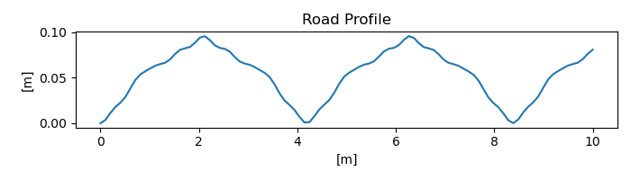
Plot the road.
r11, r22, r33, r44, r55 = [par_map[key] for key in [r1, r2, r3, r4, r5]]
rough_surface_lam = sm.lambdify((x_car, r1, r2, r3, r4, r5),
                                rough_surface(x_car), cse=True)
xx = np.linspace(0, 10, 100)
r11, r22, r33, r44, r55 = [par_map[key] for key in [r1, r2, r3, r4, r5]]
fig, ax = plt.subplots(figsize=(7, 2), layout='tight')
ax.plot(xx, rough_surface_lam(xx, r11, r22, r33, r44, r55))
ax.set_xlabel('[m]')
ax.set_ylabel('[m]')
_ = ax.set_title('Road Profile')
To be minimized:
\(\int (\dfrac{d}{dt}uz_{car})^2 dt + \text{weight} \cdot t_f\)
weight is a scalar that can be used to adjust the importance of the
speed.
weight = 1.e9


def obj(free):
    uz_dot = np.sum([free[i]**2 for i in range(6*num_nodes, 7*num_nodes)])
    return (uz_dot)*free[-1] + weight*free[-1]


def obj_grad(free):
    grad = np.zeros_like(free)
    grad[6*num_nodes:7*num_nodes] = 2*free[6*num_nodes:7*num_nodes]*free[-1]
    grad[-1] = (np.sum([free[i]**2 for i in range(6*num_nodes, 7*num_nodes)])
                + weight)
    return grad
Add the instance constraints and bounds.
instance_constraints = (
    x_car.func(t0) - 0.0,
    ux_car.func(t0) - 0.0,
    accel_street.func(t0) - 0.0,
    accel_body.func(t0) - 0.0,
    x_car.func(tf) - 10.0,
    ux_car.func(tf) - 0.0,
)

bounds = {
    h: (0.0, 1.0),
    x_car: (0.0, 10.0),
    z_wheel: (0.0, 2.0),
    ux_car: (0.0, np.inf),
    c: (0.0, np.inf),
    k: (15000, 500000),
    fx: (-50000, 50000),
    l_GW: (0.0, 1.0),
}

eom_bounds = {
    6: (0.0, 0.1),
    7: (0.85, 1.0),
}
Use an existing solution if available, else pick an initial guess and solve the problem.
prob = Problem(
    obj,
    obj_grad,
    eom,
    state_symbols,
    num_nodes,
    interval,
    known_parameter_map=par_map,
    instance_constraints=instance_constraints,
    bounds=bounds,
    eom_bounds=eom_bounds,
    time_symbol=t,
    backend='numpy',
)

fname = f'quarter_car_on_bumpy_road_{num_nodes}_nodes_solution.csv'
if os.path.exists(fname):
    # use the existing solution
    solution = np.loadtxt(fname)
else:
    # Pick a reasonable initial guess and solve the problem. Sometimes a random
    # initial guess work fine.
    np.random.seed(123)
    initial_guess = np.random.rand(prob.num_free)
    solution, info = prob.solve(initial_guess)
    print(info['status_msg'])
    print(f"Objective value, {info['obj_val']:,.2f}")
    _ = prob.plot_objective_value()
Print optimal values of the free parameters.
print('Sequence of unknown parameters',
      prob.collocator.unknown_parameters)
print(f'optimal value of dampening constant c =                  '
      f'{solution[-4]:.1f}')
print(f'optimal value of spring constant k =                     '
      f'{solution[-3]:.1f}')
print(f'optimal value of nat.  length of the wheel spring l_GW = '
      f'{solution[-2]:.2f}')
Sequence of unknown parameters (c, k, l_GW)
optimal value of dampening constant c =                  3140.6
optimal value of spring constant k =                     37667.7
optimal value of nat.  length of the wheel spring l_GW = 0.08
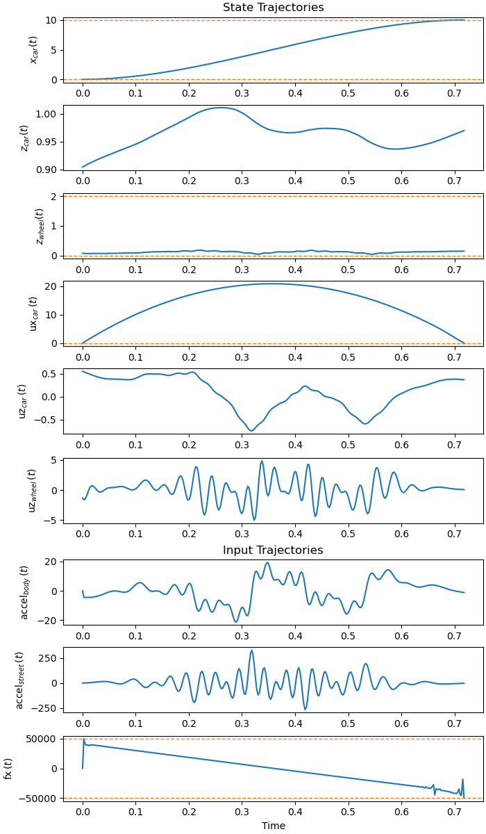
Plot the solution.
fig, axes = plt.subplots(9, 1, figsize=(7, 12), layout='constrained')
_ = prob.plot_trajectories(solution, show_bounds=True, axes=axes)
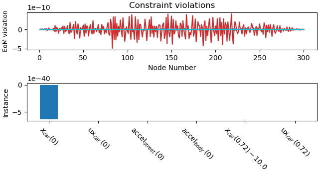
Plot the constraint violations.
_ = prob.plot_constraint_violations(solution)
Animate the Solution
fps (frames per second) is set to a higher than usual value so the fast
changing acceleration vectors can been seen more clearly.
fps = 100

state_vals, input_vals, unknown_param, h_val = prob.parse_free(solution)
t_arr = prob.time_vector(solution=solution)
state_sol = CubicSpline(t_arr, state_vals.T)
input_sol = CubicSpline(t_arr, input_vals.T)

xmin = -0.75
xmax = 0.75
ymin = -0.25
ymax = 1.25

# Average position of body and of wheel
average_body = np.mean(solution[num_nodes:2*num_nodes])
average_wheel = np.mean(solution[2*num_nodes:3*num_nodes])

# Define the points to be plotted.
coordinates = P_car.pos_from(O).to_matrix(N)
coordinates = coordinates.row_join(P_wheel.pos_from(O).to_matrix(N))

pl, pl_vals = zip(*par_map.items())
coords_lam = sm.lambdify(list(state_symbols) + list(specified_symbols) + [c, k]
                         + list(pl), coordinates, cse=True)


def init_plot():
    fig, ax = plt.subplots(figsize=(7, 7))
    ax.set_xlim(xmin, xmax)
    ax.set_ylim(ymin, ymax)
    ax.set_aspect('equal')
    ax.set_xlabel('x', fontsize=15)
    ax.set_ylabel('z', fontsize=15)

    # draw the road
    xx = np.linspace(0, 10, 200)
    street, = ax.plot(xx, rough_surface_lam(xx, r11, r22, r33, r44, r55),
                      color='black', lw=0.75)

    ax.axhline(average_body, color='black', lw=0.5, linestyle='--')
    ax.axhline(average_wheel, color='black', lw=0.5, linestyle='--')

    ax.annotate(
        f'Average height \n of the body',
        xy=(0.4, average_body),  # point to annotate
        xytext=(0.4, 0.6),  # position of the text
        arrowprops=dict(
            arrowstyle='->',
            connectionstyle='arc3,rad=0.3',  # controls curvature
            color='blue'
        ),
        fontsize=10,
        color='black',
    )

    ax.annotate(
        f'Average height of the \n center of the wheel',
        xy=(-0.4, average_wheel),  # point to annotate
        xytext=(-0.6, 0.6),  # position of the text
        arrowprops=dict(
            arrowstyle='->',
            connectionstyle='arc3,rad=0.3',  # controls curvature
            color='blue'
        ),
        fontsize=10,
        color='black',
    )

    # draw the wheel and the body and a line connecting them.
    line1 = ax.scatter([], [], color='red', marker='o', s=25)  # wheel
    line2 = ax.scatter([], [], color='red', marker='o', s=900)  # body
    line3, = ax.plot([], [], lw=2.5, color='red')  # line connecting them
    line4 = ax.scatter([], [], color='blue', marker='o', s=50)  # contact

    # draw the arrows
    # driving force
    pfeil1 = ax.quiver([], [], [], [], color='green', scale=90000, width=0.006)
    # acceleration of the wheel
    pfeil2 = ax.quiver([], [], [], [], color='blue', scale=350, width=0.006)
    # acceleration of the body
    pfeil3 = ax.quiver([], [], [], [], color='black', scale=350, width=0.006)

    circle = patches.Circle((0.1, 0.0), radius=0.1, color='red', ec='black',
                            fill=False)
    ax.add_patch(circle)

    return (fig, ax, line1, line2, line3, line4, pfeil1, pfeil2, pfeil3,
            street, circle)


# Function to update the plot for each animation frame
def update(t):
    message = (f'running time {t:.2f} sec'
               f'\n The blue arrow is the acceleration the street \n'
               f'The black arrow is the acceleration of the body \n'
               f'The green arrow is the driving force \n The video is in slow '
               f'motion')
    ax.set_title(message, fontsize=10)

    coords = coords_lam(*state_sol(t), *input_sol(t), solution[-3],
                        solution[-2], *pl_vals)
    line1.set_offsets([0, coords[2, 1]])
    line2.set_offsets([0, coords[2, 0]])
    line3.set_data([0, 0], [coords[2, 0], coords[2, 1]])
    line4.set_offsets([0, rough_surface_lam(coords[0, 0], r11, r22, r33, r44,
                                            r55)])

    xx = np.linspace(-coords[0, 0]-1, 11-coords[0, 0], 200)
    yy = np.linspace(-1, 11, 200)
    street.set_data(xx, rough_surface_lam(yy, r11, r22, r33, r44, r55))

    pfeil1.set_offsets([coords[0, 0]*0, coords[2, 0]])
    pfeil1.set_UVC(input_sol(t)[2], 0)

    pfeil2.set_offsets([-0.025, rough_surface_lam(coords[0, 0], r11, r22, r33,
                                                  r44, r55)])
    pfeil2.set_UVC(0.0, input_sol(t)[1])

    pfeil3.set_offsets([+0.05, coords[2, 0]])
    pfeil3.set_UVC(0.0, input_sol(t)[0])

    circle.set_center((0, coords[2, 1]))
Create the animation. sphinx_gallery_thumbnail_number = 4
fig, ax, line1, line2, line3, line4, pfeil1, pfeil2, pfeil3, street, circle = (
    init_plot())

animation = FuncAnimation(
    fig,
    update,
    frames=np.arange(t0, num_nodes*solution[-1], 1/fps),
    interval=12000/fps,
)

plt.show()
Total running time of the script: (0 minutes 53.535 seconds)