Block Sliding Over a Hill

Objective

• Show how to use fixed time interval and variable time interval on a very simple example.

• Show the use of backend='numpy' in the Problem class which sets up small problems faster.

Introduction

A block, modeled as a particle is sliding on a road to cross a hill. The block is subject to gravity and speed dependent viscous friction. Gravity points in the negative Y direction. A force tangential to the road is applied to the block to make it move.

Two objective functions to be minimized will be considered:

• selection = 0: time to reach the end point is minimized

• selection = 1: integral sum of the applied force is minimized

Constants

• m: mass of the block [kg]

• g: acceleration due to gravity [m/s**2]

• friction: coefficient of viscous friction [N/(m*s)]

• a, b: parameters determining the shape of the road.

States

• x: position of the block along the road [m]

• ux: speed of the block tangent to the road [m/s]

Specifieds

• F: tangential force applied to the block [N]

import numpy as np
import sympy as sm
import sympy.physics.mechanics as me
from opty import Problem
import matplotlib.pyplot as plt
from matplotlib.animation import FuncAnimation

The function below defines the shape of the road the block is sliding on.

def strasse(x, a, b):
    return a*x**2*sm.exp((b - x))

Set up Kane’s equations of motion.

N = me.ReferenceFrame('N')

O = me.Point('O')
P0 = me.Point('P0')

t = me.dynamicsymbols._t

x = me.dynamicsymbols('x')
ux = me.dynamicsymbols('u_x')
F = me.dynamicsymbols('F')

m, g, friction = sm.symbols('m, g, friction')
a, b = sm.symbols('a b')

O.set_vel(N, 0)
P0.set_pos(O, x*N.x + strasse(x, a, b)*N.y)
P0.set_vel(N, ux*N.x + strasse(x, a, b).diff(x)*ux*N.y)
bodies = [me.Particle('P0', P0, m)]

The control force and the friction are acting in the direction of the tangent at the road at the point where the particle is.

alpha = sm.atan(strasse(x, a, b).diff(x))
forces = [(P0, -m*g*N.y + F*(sm.cos(alpha)*N.x + sm.sin(alpha)*N.y) -
           friction*ux*(sm.cos(alpha)*N.x + sm.sin(alpha)*N.y))]

kd = sm.Matrix([ux - x.diff(t)])

q_ind = [x]
u_ind = [ux]

kane = me.KanesMethod(N, q_ind=q_ind, u_ind=u_ind, kd_eqs=kd)
fr, frstar = kane.kanes_equations(bodies, forces)
eom = kd.col_join(fr + frstar)
sm.trigsimp(eom)
sm.pprint(eom)

speicher = (x, ux, F)

⎡                                                                              ↪
⎢                                                                              ↪
⎢                                                                              ↪
⎢                                                                              ↪
⎢                                                                              ↪
⎢                    friction⋅uₓ(t)                        ⎛     2     b - x(t ↪
⎢- ─────────────────────────────────────────────────── - m⋅⎝- a⋅x (t)⋅ℯ        ↪
⎢      _______________________________________________                         ↪
⎢     ╱                                         2                              ↪
⎢    ╱  ⎛   2     b - x(t)             b - x(t)⎞                               ↪
⎣  ╲╱   ⎝a⋅x (t)⋅ℯ         - 2⋅a⋅x(t)⋅ℯ        ⎠  + 1                          ↪

↪                                                                              ↪
↪                                                                              ↪
↪                                                                              ↪
↪                                                                              ↪
↪                                                                              ↪
↪ )             b - x(t)⎞ ⎛         2     b - x(t)                   b - x(t)  ↪
↪   + 2⋅a⋅x(t)⋅ℯ        ⎠⋅⎝a⋅uₓ(t)⋅x (t)⋅ℯ         - 4⋅a⋅uₓ(t)⋅x(t)⋅ℯ          ↪
↪                                                                              ↪
↪                                                                              ↪
↪                                                                              ↪
↪                                                                              ↪

↪                                                                              ↪
↪                                                                       uₓ(t)  ↪
↪                                                                              ↪
↪                                                                              ↪
↪                                  ⎛                                           ↪
↪              b - x(t)⎞           ⎜⎛     2     b - x(t)             b - x(t)⎞ ↪
↪ + 2⋅a⋅uₓ(t)⋅ℯ        ⎠⋅uₓ(t) - m⋅⎝⎝- a⋅x (t)⋅ℯ         + 2⋅a⋅x(t)⋅ℯ        ⎠ ↪
↪                                                                              ↪
↪                                                                              ↪
↪                                                                              ↪
↪                                                                              ↪

↪   d                                                                          ↪
↪ - ──(x(t))                                                                   ↪
↪   dt                                                                         ↪
↪                                                                              ↪
↪ 2    ⎞                                                        ⎛         ⎛    ↪
↪      ⎟ d           ⎛     2     b - x(t)             b - x(t)⎞ ⎜friction⋅⎝a⋅x ↪
↪   + 1⎠⋅──(uₓ(t)) + ⎝- a⋅x (t)⋅ℯ         + 2⋅a⋅x(t)⋅ℯ        ⎠⋅⎜───────────── ↪
↪        dt                                                     ⎜      _______ ↪
↪                                                               ⎜     ╱        ↪
↪                                                               ⎜    ╱  ⎛   2  ↪
↪                                                               ⎝  ╲╱   ⎝a⋅x ( ↪

↪                                                                              ↪
↪                                                                              ↪
↪                                                                              ↪
↪                                                                              ↪
↪ 2     b - x(t)             b - x(t)⎞                  ⎛   2     b - x(t)     ↪
↪  (t)⋅ℯ         - 2⋅a⋅x(t)⋅ℯ        ⎠⋅uₓ(t)            ⎝a⋅x (t)⋅ℯ         - 2 ↪
↪ ────────────────────────────────────────── - g⋅m - ───────────────────────── ↪
↪ ________________________________________               _____________________ ↪
↪                                   2                   ╱                      ↪
↪     b - x(t)             b - x(t)⎞                   ╱  ⎛   2     b - x(t)   ↪
↪ t)⋅ℯ         - 2⋅a⋅x(t)⋅ℯ        ⎠  + 1            ╲╱   ⎝a⋅x (t)⋅ℯ         - ↪

↪                                                                              ↪
↪                                                                              ↪
↪                                                                              ↪
↪                                                                              ↪
↪          b - x(t)⎞        ⎞                                                  ↪
↪ ⋅a⋅x(t)⋅ℯ        ⎠⋅F(t)   ⎟                          F(t)                    ↪
↪ ──────────────────────────⎟ + ────────────────────────────────────────────── ↪
↪ __________________________⎟       __________________________________________ ↪
↪                     2     ⎟      ╱                                         2 ↪
↪            b - x(t)⎞      ⎟     ╱  ⎛   2     b - x(t)             b - x(t)⎞  ↪
↪  2⋅a⋅x(t)⋅ℯ        ⎠  + 1 ⎠   ╲╱   ⎝a⋅x (t)⋅ℯ         - 2⋅a⋅x(t)⋅ℯ        ⎠  ↪

↪      ⎤
↪      ⎥
↪      ⎥
↪      ⎥
↪      ⎥
↪      ⎥
↪ ─────⎥
↪ _____⎥
↪      ⎥
↪      ⎥
↪  + 1 ⎦

Store the results of the two optimizations for later plotting

solution_list = []
prob_list = []
info_list = []

Define the known parameters.

par_map = {}
par_map[m] = 1.0
par_map[g] = 9.81
par_map[friction] = 0.0
par_map[a] = 1.5
par_map[b] = 2.5

num_nodes = 150
fixed_duration = 6.0  # seconds

Set up the optimization problems and solve them.

for selection in (0, 1):
    state_symbols = (speicher[0], speicher[1])
    num_states = len(state_symbols)
    constant_symbols = (m, g, friction, a, b)
    specified_symbols = (speicher[2], )

    if selection == 1:  # minimize integral of force magnitude
        duration = fixed_duration
        interval_value = duration/(num_nodes - 1)

        def obj(free):
            Fx = free[num_states*num_nodes:(num_states + 1)*num_nodes]
            return interval_value*np.sum(Fx**2)

        def obj_grad(free):
            grad = np.zeros_like(free)
            l1 = num_states*num_nodes
            l2 = (num_states + 1)*num_nodes
            grad[l1: l2] = 2.0*free[l1:l2]*interval_value
            return grad

    elif selection == 0:  # minimize total duration
        h = sm.symbols('h')
        duration = (num_nodes - 1)*h
        interval_value = h

        def obj(free):
            return free[-1]

        def obj_grad(free):
            grad = np.zeros_like(free)
            grad[-1] = 1.0
            return grad

    t0, tf = 0.0, duration

    initial_guess = np.ones((num_states +
                             len(specified_symbols))*num_nodes)*0.01
    if selection == 0:
        initial_guess = np.hstack((initial_guess, 0.02))

    initial_state_constraints = {x: 0.0, ux: 0.0}
    final_state_constraints = {x: 10.0, ux: 0.0}

    instance_constraints = (
        tuple(xi.subs({t: t0}) - xi_val for xi, xi_val in
              initial_state_constraints.items()) +
        tuple(xi.subs({t: tf}) - xi_val for xi, xi_val in
              final_state_constraints.items())
    )

    bounds = {F: (-10., 15.),
              x: (initial_state_constraints[x], final_state_constraints[x]),
              ux: (0., 100)}
    if selection == 0:
        bounds[h] = (1.e-5, 1.)

    prob = Problem(
        obj,
        obj_grad,
        eom,
        state_symbols,
        num_nodes,
        interval_value,
        known_parameter_map=par_map,
        instance_constraints=instance_constraints,
        bounds=bounds,
        backend='numpy',
    )

    solution, info = prob.solve(initial_guess)
    solution_list.append(solution)
    info_list.append(info)
    prob_list.append(prob)

Animate the solutions and plot the results.

def drucken(selection, fig, ax, video=True):
    solution = solution_list[selection]

    if selection == 0:
        duration = (num_nodes - 1)*solution[-1]
        times = prob.time_vector(solution=solution)
    else:
        duration = fixed_duration
        times = prob.time_vector()
    interval_value = duration/(num_nodes - 1)

    strasse1 = strasse(x, a, b)
    strasse_lam = sm.lambdify((x, a, b), strasse1, cse=True)

    P0_x = solution[:num_nodes]
    P0_y = strasse_lam(P0_x, par_map[a], par_map[b])

    # find the force vector applied to the block
    alpha = sm.atan(strasse(x, a, b).diff(x))
    Pfeil = [F*sm.cos(alpha),  F*sm.sin(alpha)]
    Pfeil_lam = sm.lambdify((x, F, a, b), Pfeil, cse=True)

    l1 = num_states*num_nodes
    l2 = (num_states + 1)*num_nodes
    Pfeil_x = Pfeil_lam(P0_x, solution[l1: l2], par_map[a], par_map[b])[0]
    Pfeil_y = Pfeil_lam(P0_x, solution[l1: l2], par_map[a], par_map[b])[1]

    # needed to give the picture the right size.
    xmin = np.min(P0_x)
    xmax = np.max(P0_x)
    ymin = np.min(P0_y)
    ymax = np.max(P0_y)

    def initialize_plot():
        ax.set_xlim(xmin-1, xmax + 1.)
        ax.set_ylim(ymin-1, ymax + 1.)
        ax.set_aspect('equal')
        ax.set_xlabel('X-axis [m]')
        ax.set_ylabel('Y-axis [m]')

        if selection == 0:
            msg = 'The speed is optimized'
        else:
            msg = 'The energy optimized'

        ax.grid()
        strasse_x = np.linspace(xmin, xmax, 100)
        ax.plot(strasse_x, strasse_lam(strasse_x, par_map[a], par_map[b]),
                color='black', linestyle='-', linewidth=1)
        ax.axvline(initial_state_constraints[x], color='r', linestyle='--',
                   linewidth=1)
        ax.axvline(final_state_constraints[x], color='green', linestyle='--',
                   linewidth=1)

        # Initialize the block and the arrow
        line1, = ax.plot([], [], color='blue', marker='o', markersize=12)
        pfeil = ax.quiver([], [], [], [], color='green', scale=35, width=0.004)

        return line1, pfeil, msg

    line1, pfeil, msg = initialize_plot()

    # Function to update the plot for each animation frame
    def update(frame):
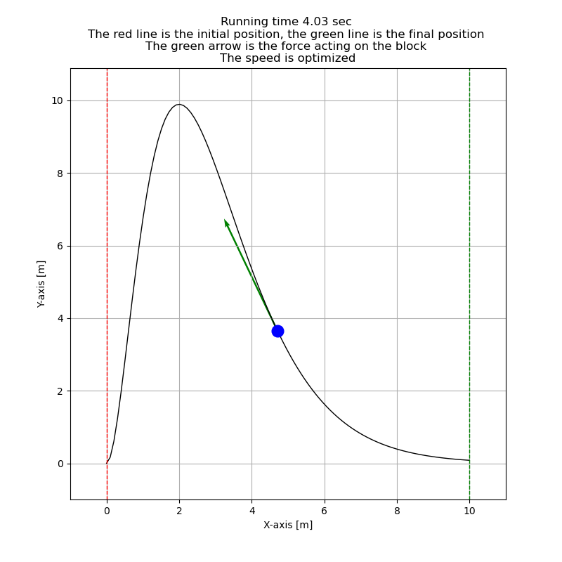
        message = (f'Running time {times[frame]:.2f} sec \n'
                   'The red line is the initial position, the green line is '
                   'the final position \n'
                   'The green arrow is the force acting on the block \n'
                   f'{msg}')
        ax.set_title(message, fontsize=12)

        line1.set_data([P0_x[frame]], [P0_y[frame]])
        pfeil.set_offsets([P0_x[frame], P0_y[frame]])
        pfeil.set_UVC(Pfeil_x[frame], Pfeil_y[frame])
        return line1, pfeil

    if video:
        animation = FuncAnimation(fig, update, frames=range(len(P0_x)),
                                  interval=1000*interval_value)
    else:
        animation = None

    return animation, update

Below the results of minimized duration are shown.

selection = 0
print('Message from optimizer:', info_list[selection]['status_msg'])
print(f'Optimal h value is: {solution_list[selection][-1]:.3f}')

Message from optimizer: b'Algorithm terminated successfully at a locally optimal point, satisfying the convergence tolerances (can be specified by options).'
Optimal h value is: 0.027

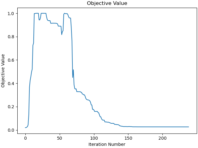
_ = prob_list[selection].plot_objective_value()

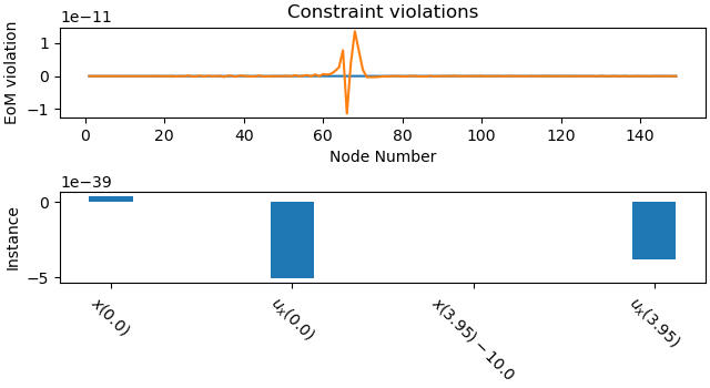
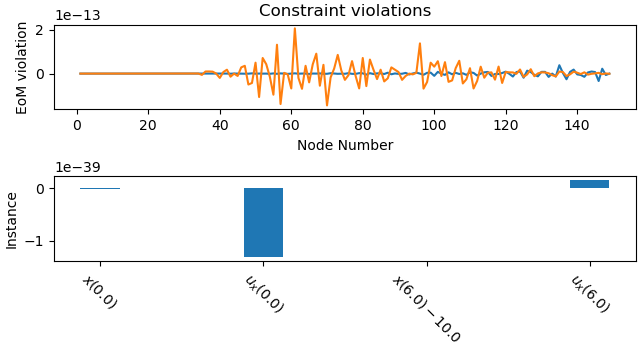
Plot errors in the solution.

_ = prob_list[selection].plot_constraint_violations(solution_list[selection])

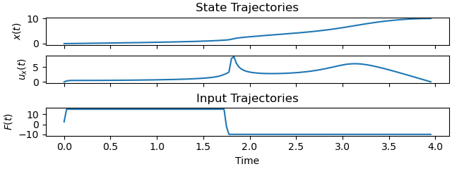
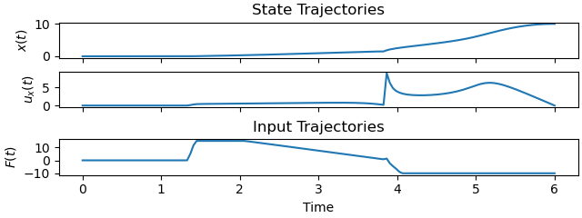
Plot the trajectories of the block.

_ = prob_list[selection].plot_trajectories(solution_list[selection])

Animate the solution.

fig, ax = plt.subplots(figsize=(8, 8))
anim, _ = drucken(selection, fig, ax)

Once Loop Reflect

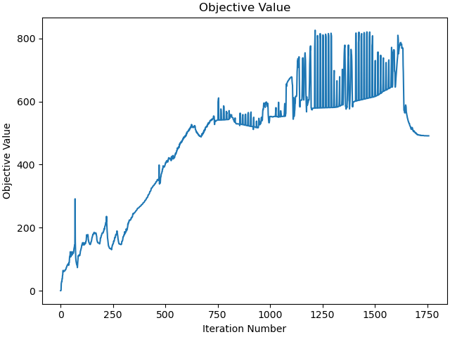
Now the results of minimized energy are shown.

selection = 1
print('Message from optimizer:', info_list[selection]['status_msg'])

Message from optimizer: b'Algorithm terminated successfully at a locally optimal point, satisfying the convergence tolerances (can be specified by options).'

_ = prob_list[selection].plot_objective_value()

Plot errors in the solution.

_ = prob_list[selection].plot_constraint_violations(solution_list[selection])

Plot the trajectories of the block.

_ = prob_list[selection].plot_trajectories(solution_list[selection])

Animate the solution.

fig, ax = plt.subplots(figsize=(8, 8))
anim, _ = drucken(selection, fig, ax)

Once Loop Reflect

A frame from the animation.

fig, ax = plt.subplots(figsize=(8, 8))
_, update = drucken(0, fig, ax, video=False)
update(100)

plt.show()