Parameter Identification from Noncontiguous Measurements

In parameter estimation it is common to collect measurements of a system’s trajectories from distinct experiments. For example, if you are identifying the parameters of a mass-spring-damper system, you may excite the system with different initial conditions multiple times and measure the position of the mass. The data cannot simply be stacked end-to-end in time and the identification run because the measurement data would be discontinuous between each measurement trial.

A workaround in opty is to create a set of differential equations with unique state variables for each measurement trial that all share the same constant parameters. You can then identify the parameters from all measurement trials simultaneously by passing the uncoupled differential equations to opty.

Mass-spring-damper Example

The position of a simple system consisting of a mass connected to a fixed point by a spring and a damper is simulated and recorded as noisy measurements. The spring constant and the damping coefficient will be identified.

State Variables

• \(x_1\): position of the mass of the first measurement trial [m]

• \(x_2\): position of the mass of the second measurement trial [m]

• \(x_3\): position of the mass of the third measurement trial [m]

• \(x_4\): position of the mass of the fourth measurement trial [m]

• \(u_1\): speed of the mass of the first measurement trial [m/s]

• \(u_2\): speed of the mass of the second measurement trial [m/s]

• \(u_3\): speed of the mass of the third measurement trial [m/s]

• \(u_4\): speed of the mass of the fourth measurement trial [m/s]

Parameters

• \(m\): mass [kg]

• \(c\): linear damping coefficient [Ns/m]

• \(k\): linear spring constant [N/m]

• \(l_0\): natural length of the spring [m]

import sympy as sm
import sympy.physics.mechanics as me
import numpy as np
from scipy.integrate import solve_ivp
from opty import Problem
import matplotlib.pyplot as plt

Equations of Motion

Set up the four sets of equations of motion, one for each of the four measurements.

x1, x2, x3, x4 = me.dynamicsymbols('x1, x2, x3, x4')
u1, u2, u3, u4 = me.dynamicsymbols('u1, u2, u3, u4')
m, c, k, l0 = sm.symbols('m, c, k, l0')
t = me.dynamicsymbols._t

eom = sm.Matrix([
    x1.diff(t) - u1,
    x2.diff(t) - u2,
    x3.diff(t) - u3,
    x4.diff(t) - u4,
    m*u1.diff(t) + c*u1 + k*(x1 - l0),
    m*u2.diff(t) + c*u2 + k*(x2 - l0),
    m*u3.diff(t) + c*u3 + k*(x3 - l0),
    m*u4.diff(t) + c*u4 + k*(x4 - l0),
])

sm.pprint(eom)

⎡                   d                   ⎤
⎢          -u₁(t) + ──(x₁(t))           ⎥
⎢                   dt                  ⎥
⎢                                       ⎥
⎢                   d                   ⎥
⎢          -u₂(t) + ──(x₂(t))           ⎥
⎢                   dt                  ⎥
⎢                                       ⎥
⎢                   d                   ⎥
⎢          -u₃(t) + ──(x₃(t))           ⎥
⎢                   dt                  ⎥
⎢                                       ⎥
⎢                   d                   ⎥
⎢          -u₄(t) + ──(x₄(t))           ⎥
⎢                   dt                  ⎥
⎢                                       ⎥
⎢                              d        ⎥
⎢c⋅u₁(t) + k⋅(-l₀ + x₁(t)) + m⋅──(u₁(t))⎥
⎢                              dt       ⎥
⎢                                       ⎥
⎢                              d        ⎥
⎢c⋅u₂(t) + k⋅(-l₀ + x₂(t)) + m⋅──(u₂(t))⎥
⎢                              dt       ⎥
⎢                                       ⎥
⎢                              d        ⎥
⎢c⋅u₃(t) + k⋅(-l₀ + x₃(t)) + m⋅──(u₃(t))⎥
⎢                              dt       ⎥
⎢                                       ⎥
⎢                              d        ⎥
⎢c⋅u₄(t) + k⋅(-l₀ + x₄(t)) + m⋅──(u₄(t))⎥
⎣                              dt       ⎦

Generate Noisy Measurement Data

Create four sets of measurements with different initial conditions. To get the measurements, the equations of motion are integrated, and then noise is added to each point in time of the solution.

rhs = sm.Matrix([
    u1,
    u2,
    u3,
    u4,
    1/m*(-c*u1 - k*(x1 - l0)),
    1/m*(-c*u2 - k*(x2 - l0)),
    1/m*(-c*u3 - k*(x3 - l0)),
    1/m*(-c*u4 - k*(x4 - l0)),
])
states = [x1, x2, x3, x4, u1, u2, u3, u4]
parameters = [m, c, k, l0]
par_vals = [1.0, 0.25, 1.0, 1.0]

eval_rhs = sm.lambdify(states + parameters, rhs)

t0, tf = 0.0, 20.0
num_nodes = 500
times = np.linspace(t0, tf, num=num_nodes)

measurements = []
np.random.seed(123)
for i in range(4):
    x0 = 4.0*np.random.randn(8)
    sol = solve_ivp(lambda t, x, p: eval_rhs(*x, *p).squeeze(),
                    (t0, tf), x0, t_eval=times, args=(par_vals,))
    measurements.append(sol.y[0, :] +
                        2.0*np.random.randn(len(sol.t)))
measurements = np.array(measurements)

print(measurements.shape)

(4, 500)

Setup the Identification Problem

The goal is to identify the damping coefficient \(c\) and the spring constant \(k\). The objective \(J\) is to minimize the least square difference in the optimal simulation as compared to the measurements. If some measurement is considered more reliable, its weight \(w\) may be increased relative to the other measurements.

\[\begin{split}J(x_1, x_2, x_3, x_4) = \\ \int_{t_0}^{t_f} \left( w_1 (x_1 - x_1^m)^2 + w_2 (x_2 - x_2^m)^2 + w_3 (x_3 - x_3^m)^2 + w_4 (x_4 - x_4^m)^2 \right) dt\end{split}\]

interval_value = (tf - t0) / (num_nodes - 1)

w = [1.0, 1.0, 1.0, 1.0]


def obj(free):
    return interval_value*np.sum(
        w[0]*(free[0*num_nodes:1*num_nodes] - measurements[0])**2 +
        w[1]*(free[1*num_nodes:2*num_nodes] - measurements[1])**2 +
        w[2]*(free[2*num_nodes:3*num_nodes] - measurements[2])**2 +
        w[3]*(free[3*num_nodes:4*num_nodes] - measurements[3])**2)


def obj_grad(free):
    grad = np.zeros_like(free)
    grad[:num_nodes] = 2*w[0]*interval_value*(
        free[0*num_nodes:1*num_nodes] - measurements[0])
    grad[num_nodes:2*num_nodes] = 2*w[1]*interval_value*(
        free[1*num_nodes:2*num_nodes] - measurements[1])
    grad[2*num_nodes:3*num_nodes] = 2*w[2]*interval_value*(
        free[2*num_nodes:3*num_nodes] - measurements[2])
    grad[3*num_nodes:4*num_nodes] = 2*w[3]*interval_value*(
        free[3*num_nodes:4*num_nodes] - measurements[3])
    return grad

By not including \(c\) and \(k\) in the parameter map, they will be treated as unknown parameters.

par_map = {m: par_vals[0], l0: par_vals[3]}
print(par_map)

{m: 1.0, l0: 1.0}

bounds = {
    c: (0.01, 2.0),
    k: (0.1, 10.0),
}

problem = Problem(
    obj,
    obj_grad,
    eom,
    states,
    num_nodes,
    interval_value,
    known_parameter_map=par_map,
    time_symbol=me.dynamicsymbols._t,
    integration_method='midpoint',
    bounds=bounds,
)

Create an Initial Guess

It is reasonable to use the measurements as initial guess for the states because they would be available. Here, only the measurements of the position are used and the speeds are set to zero. The last two values are the guesses for \(c\) and \(k\), respectively.

initial_guess = np.hstack((np.array(measurements).flatten(),  # x
                           np.zeros(4*num_nodes),  # u
                           [0.1, 3.0]))  # c, k

Solve the Optimization Problem

solution, info = problem.solve(initial_guess)
print(info['status_msg'])

b'Algorithm terminated successfully at a locally optimal point, satisfying the convergence tolerances (can be specified by options).'

_ = problem.plot_objective_value()

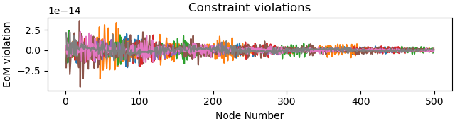
_ = problem.plot_constraint_violations(solution)

The identified parameters are:

print(f'Estimate of damping coefficient is {solution[-2]: 1.2f}')
print(f'Estimate of the spring constant is {solution[-1]: 1.2f}')

Estimate of damping coefficient is  0.25
Estimate of the spring constant is  1.01

Plot the Measurements and the Estimated Trajectories

fig, ax = plt.subplots(8, 1, figsize=(6, 8), sharex=True)
for i in range(4):
    ax[i].plot(times, measurements[i])
problem.plot_trajectories(solution, axes=ax)

plt.show()