Mississippi Steamboat

Objectives

• Show the usage of opty’s variable node time interval feature.

• Show an objective function which is a weighted average of the time and of the energy needed.

Introduction

A boat is modeled as a rectangular plate with length \(a_S\) and width \(b_S\). It has a mass \(m_S\) and is modeled as a rigid body. Water wheels are attached to the boat on the left and right side. The wheels have radius \(r_W\) and mass \(m_W\) and are modeled as rigid bodies. By running the wheels at different speeds, the boat can be steered. The water speed is assumed to be zero. Gravity, in the negative Z direction, is unimportant here, therefore disregarded.

Notes

The equations of motion might be of interest.

Constants

• \(m_S\): mass of the steamboat [kg]

• \(m_W\): mass of the wheels [kg]

• \(r_W\): radius of the wheel [m]

• \(a_S\): length of the steamboat [m]

• \(b_S\): width of the steamboat [m]

• \(c_W\): drag coefficient at wheels [kg/m^2]

• \(c_S\): drag coefficient at steamboat [kg/m^2]

States

• \(x\): X - position of the center of the steamboat [m]

• \(y\): Y - position of the center of the steamboat [m]

• \(q_S\): angle of the steamboat [rad]

• \(q_{LW}\): angle of the left wheel [rad]

• \(q_{RW}\): angle of the right wheel [rad]

• \(u_x\): speed of the steamboat in X direction [m/s]

• \(u_y\): speed of the steamboat in Y direction [m/s]

• \(u_S\): angular speed of the steamboat [rad/s]

• \(u_{LW}\): angular speed of the left wheel [rad/s]

• \(u_{RW}\): angular speed of the right wheel [rad/s]

Specifieds

• \(t_{LW}\): torque applied to the left wheel [Nm]

• \(t_{RW}\): torque applied to the right wheel [Nm]

import os
import numpy as np
import sympy as sm
from scipy.interpolate import CubicSpline
import sympy.physics.mechanics as me
from opty.direct_collocation import Problem
import matplotlib.pyplot as plt
from matplotlib.animation import FuncAnimation
from matplotlib.patches import Rectangle

Set up the Equations of Motion

Set up the geometry of the system.

• \(N\): inertial frame of reference

• \(O\): origin of the inertial frame of reference

• \(A_S\): body fixed frame of the steamboat

• \(A_{LW}\): body fixed frame of the left wheel

• \(A_{RW}\): body fixed frame of the right wheel

• \(A^{o}_S\): center of the steamboat

• \(A^{o}_{LW}\): center of the left wheel

• \(A^{o}_{RW}\): center of the right wheel

• \(FP_{LW}\): point where the force due to rotation of the left wheel is applied

• \(FP_{RW}\): point where the force due to rotation of the right wheel is applied

N, AS, ALW, ARW = sm.symbols('N, AS, ALW, ARW', cls=me.ReferenceFrame)
AoS, AoLW, AoRW = sm.symbols('AoS, AoLW, AoRW', cls=me.Point)
O, FPLW, FPRW = sm.symbols('O, FPLW, FPRW', cls=me.Point)

q, x, y, qLW, qRW = me.dynamicsymbols('q, x, y, qLW, qRW')
u, ux, uy, uLW, uRW = me.dynamicsymbols('u, ux, uy, uLW, uRW')
tLW, tRW = me.dynamicsymbols('tLW, tRW')

mS, mW, rW, aS, bS, cS, cW = sm.symbols('mS, mW, rW, aS, bS, cS, cW', real=True)

t = me.dynamicsymbols._t
O.set_vel(N, 0)

AS.orient_axis(N, q, N.z)
AS.set_ang_vel(N, u*N.z)
ALW.orient_axis(AS, qLW, AS.x)
ALW.set_ang_vel(AS, uLW*AS.x)
ARW.orient_axis(AS, qRW, AS.x)
ARW.set_ang_vel(AS, uRW*AS.x)

AoS.set_pos(O, x*N.x + y*N.y)
AoS.set_vel(N, ux*N.x + uy*N.y)
AoLW.set_pos(AoS, -1.1*bS*AS.x)
AoLW.v2pt_theory(AoS, N, AS)
AoRW.set_pos(AoS, 1.1*bS*AS.x)
AoRW.v2pt_theory(AoS, N, AS)

FPLW.set_pos(AoLW, -rW*N.z)
FPLW.set_vel(N, AoLW.vel(N) + uLW*AS.x.cross(-rW*N.z))
FPRW.set_pos(AoRW, -rW*N.z)
FPRW.set_vel(N, AoRW.vel(N) + uRW*AS.x.cross(-rW*N.z))

Set up the drag forces acting on the boat.

The drag force acting on a body moving in a fluid is given by \(F_D = -\dfrac{1}{2} \rho C_D A | \bar v|^2 \hat v\), where \(C_D\) is the drag coefficient, \(\bar v\) is the velocity, \(\rho\) is the density of the fluid, \(\hat v\) is the unit vector of the velocity of the body and \(A\) is the cross section area of the body facing the flow. This may be found here:

https://courses.lumenlearning.com/suny-physics/chapter/5-2-drag-forces/

\(\dfrac{1}{2} \rho C_D\) are lumped into a single constant \(c\). (In the code below, \(c_S\) for the steamboat and \(c_W\) for the wheels will be used.) In order to avoid numerical issues with .normalize(), sm.sqrt(..) the following will be used:

\(F_{D_x} = -c A (\hat{A}.x \cdot \bar v)^2 \cdot \operatorname{sgn} (\hat{A}.x \cdot \bar v) \hat{A}.x\) \(F_{D_y} = -c A (\hat{A}.y \cdot \bar v)^2 \cdot \operatorname{sgn} (\hat{A}.y \cdot \bar v) \hat{A}.y\)

As an (infinitely often) differentiable approximation of the sign function, the fairly standard approximation will be:

\(\operatorname{sgn}(x) \approx \tanh( \alpha \cdot x )\) with \(\alpha \gg 1\)

helpx = AoS.vel(N).dot(AS.x)
helpy = AoS.vel(N).dot(AS.y)

FDx = -cS*aS*(helpx**2)*sm.tanh(20*helpx)*AS.x
FDy = -cS*bS*(helpy**2)*sm.tanh(20*helpy)*AS.y
forces = [(AoS, FDx + FDy)]

Set up the forces acting on the wheels. The drag forces are similar to above, except that these forces act only in the AS.y direction.

helpy = FPLW.vel(N).dot(AS.y)
FLW = -cW*rW*(helpy**2)*sm.tanh(20*helpy)*AS.y

helpy = FPRW.vel(N).dot(AS.y)
FRW = -cW*rW*(helpy**2)*sm.tanh(20*helpy)*AS.y

forces.append((AoLW, FLW))
forces.append((AoRW, FRW))

forces.append((ALW, tLW*AS.x + (-rW*N.z).cross(FLW)))
forces.append((ARW, tRW*AS.x + (-rW*N.z).cross(FRW)))

If \(u \neq 0\), the boat will rotate and a drag torque will act on it.

Tdrag = -cS*aS * u*AS.z.cross(AS.y)
forces.append((AS, Tdrag))

If \(u \neq 0\), the boat will rotate and a drag torque will act on it. Looking at the situation from the center of the boat to its bow: At a distance \(r\) from the center, The speed of a point a r is \(u \cdot r\). The area is \(dr\), hence the force is \(-c_S (u \cdot r)^2 dr\). The leverage at this point is \(r\), hence the torque is \(-c_S (u \cdot r)^2 \cdot r dr\). Hence total torque is: \(-c_S u^2 \int_{0}^{a_S/2} r^3 \, dr\) = \(\frac{1}{4} c_S u^2 \frac{a_S}{16}\)

The same is from the center to the stern, hence the total torque is \(\frac{1}{32} c_S u^2 a_S^4\). Same again across the front, with \(b_S\) instead of \(a_S\), hence the total torque is \(\frac{1}{32} c_S u^2 b_S^4\).

tB = -cS*u**2*(aS**4 + bS**4)/32 * sm.tanh(20*u) * N.z
forces.append((AS, tB))

Set up the rigid bodies.

iXX = 0.5*mW*rW**2
iYY = 0.25*mW*rW**2
iZZ = iYY
I1 = me.inertia(ALW, iXX, iYY, iZZ)
I2 = me.inertia(ARW, iXX, iYY, iZZ)
left_wheel = me.RigidBody('left_wheel', AoLW, ALW, mW, (I1, AoLW))
right_wheel = me.RigidBody('right_wheel', AoRW, ARW, mW, (I2, AoRW))

iZZ = 1/12 * mS*(aS**2 + bS**2)
I3 = me.inertia(AS, 0, 0, iZZ)
boat = me.RigidBody('boat', AoS, AS, mS, (I3, AoS))

bodies = [boat, left_wheel, right_wheel]

Set up Kane’s equations of motion.

q_ind = [q, x, y, qLW, qRW]
u_ind = [u, ux, uy, uLW, uRW]
kd = sm.Matrix([i - j.diff(t) for j, i in zip(q_ind, u_ind)])

KM = me.KanesMethod(N,
                    q_ind=q_ind,
                    u_ind=u_ind,
                    kd_eqs=kd,
                    )

fr, frstar = KM.kanes_equations(bodies, forces)
eom = kd.col_join(fr + frstar)
print(f'The equations of motion containt {sm.count_ops(eom)} operations.')

The equations of motion containt 702 operations.

Set up the Optimization Problem and Solve It

state_symbols = [q, x, y, qLW, qRW, u, ux, uy, uLW, uRW]
specified_symbols = [tLW, tRW]
constant_symbols = [mS, mW, rW, aS, bS, cS, cW]
num_nodes = 251
h = sm.symbols('h')

Specify the known symbols.

par_map = {}
par_map[mS] = 10.0
par_map[mW] = 1.0
par_map[rW] = 1.0
par_map[aS] = 5.0
par_map[bS] = 1.0
par_map[cS] = 0.75
par_map[cW] = 0.75

Set up the objective function and its gradient. The objective function to be minimized is:

\(\text{obj} = \int_{t_0}^{t_f} \left( t_{LW}^2 + t_{RW}^2 \right) \, dt + \text{weight} \cdot h\)

where weight > 0 is the relative importance of the duration of the motion, and h > 0.

weight = 1.0e7
def obj(free):
    t1 = free[10 * num_nodes: 11 * num_nodes]
    t2 = free[11 * num_nodes: 12 * num_nodes]
    return free[-1] * (np.sum(t1**2) + np.sum(t2**2)) + free[-1] * weight

def obj_grad(free):
    grad = np.zeros_like(free)
    grad[10*num_nodes: 11*num_nodes] = 2.0*free[-1]*free[10*num_nodes: 11*num_nodes]
    grad[11*num_nodes: 12*num_nodes] = 2.0*free[-1]*free[11*num_nodes: 12*num_nodes]
    grad[-1] = weight
    return grad

duration = (num_nodes - 1)*h
t0, tf = 0.0, duration
interval_value = h

Set up the instance constraints, the bounds and Problem.

initial_state_constraints = {
    q: -np.pi/2.,
    x: 0.0,
    y: 0.0,
    qLW: 0.0,
    qRW: 0.0,
    u: 0.0,
    ux: 0.0,
    uy: 0.0,
    uLW: 0.0,
    uRW: 0.0,
}

final_state_constraints = {
    q: -np.pi/2.,
    x: 10,
    y: 10,
    u: 0.0,
    ux: 0.0,
    uy: 0.0,
}

instance_constraints = (
    q.subs({t: t0}) - initial_state_constraints[q],
    x.subs({t: t0}) - initial_state_constraints[x],
    y.subs({t: t0}) - initial_state_constraints[y],
    qLW.subs({t: t0}) - initial_state_constraints[qLW],
    qRW.subs({t: t0}) - initial_state_constraints[qRW],
    u.subs({t: t0}) - initial_state_constraints[u],
    ux.subs({t: t0}) - initial_state_constraints[ux],
    uy.subs({t: t0}) - initial_state_constraints[uy],
    uLW.subs({t: t0}) - initial_state_constraints[uLW],
    uRW.subs({t: t0}) - initial_state_constraints[uRW],
    q.subs({t: tf}) - final_state_constraints[q],
    x.subs({t: tf}) - final_state_constraints[x],
    y.subs({t: tf}) - final_state_constraints[y],
    u.subs({t: tf}) - final_state_constraints[u],
    ux.subs({t: tf}) - final_state_constraints[ux],
    uy.subs({t: tf}) - final_state_constraints[uy],
)

limit_torque = 25.
bounds = {
    tLW: (-limit_torque, limit_torque),
    tRW: (-limit_torque, limit_torque),
    h: (0.0, 1.0),
}

prob = Problem(
    obj,
    obj_grad,
    eom,
    state_symbols,
    num_nodes,
    interval_value,
    time_symbol=t,
    known_parameter_map=par_map,
    instance_constraints=instance_constraints,
    bounds=bounds,
    backend='numpy',
)

Pick a reasonable initial guess and solve the problem, if needed.

i1 = list(np.zeros(num_nodes))
i2 = list(np.linspace(initial_state_constraints[x], final_state_constraints[x],
    num_nodes))
i3 = list(np.linspace(initial_state_constraints[y], final_state_constraints[y],
    num_nodes))
i4 = list(np.zeros(9*num_nodes))
initial_guess = np.array(i1 + i2 + i3 + i4 + [0.01])

# Use given solution, if available else use the initial guess given above.
fname = f'mississippi_steamboat_{num_nodes}_nodes_solution.csv'

if os.path.exists(fname):
    # use the given solution
    solution = np.loadtxt(fname)
else:
    # calculate a solution
    for _ in range(3):
        solution, info = prob.solve(initial_guess)
        print('Message from optimizer:', info['status_msg'])
        print(f'Optimal h value is: {solution[-1]:.3f} sec')

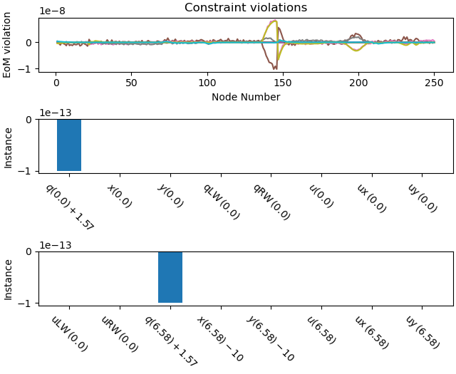
Plot errors in the solution.

_ = prob.plot_constraint_violations(solution)

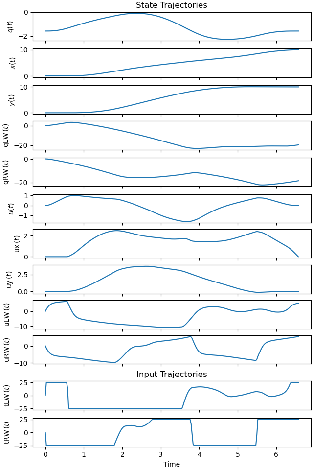
Plot the trajectories of the solution.

_ = prob.plot_trajectories(solution)

Animate the Solution

fps = 13


def add_point_to_data(line, x, y):
    # to trace the path of the point.
    old_x, old_y = line.get_data()
    line.set_data(np.append(old_x, x), np.append(old_y, y))


state_vals, input_vals, _, h_val = prob.parse_free(solution)
t_arr = prob.time_vector(solution=solution)
state_sol = CubicSpline(t_arr, state_vals.T)
input_sol = CubicSpline(t_arr, input_vals.T)

xmin = initial_state_constraints[x] - par_map[aS]/1.75
xmax = final_state_constraints[x] + par_map[aS]/1.75
ymin = initial_state_constraints[y] - par_map[aS]/1.75
ymax = final_state_constraints[y] + par_map[aS]/1.75

# additional points to plot the water wheels and the torque
pLB, pLF, pRB, pRF, tL, tR, S1, S2 = sm.symbols('pLB pLF pRB pRF tL, tR S1 S2',
    cls=me.Point)
pLB.set_pos(AoLW, -rW*AS.y)
pLF.set_pos(AoLW, rW*AS.y)
pRB.set_pos(AoRW, -rW*AS.y)
pRF.set_pos(AoRW, rW*AS.y)
tL.set_pos(O, tLW*AS.x)
tR.set_pos(O, tRW*AS.x)
S1.set_pos(AoLW, par_map[bS]/15*AS.y)
S2.set_pos(AoRW, -par_map[bS]/15 *AS.y)

coordinates = AoS.pos_from(O).to_matrix(N)
for point in (AoLW, AoRW, pLB, pLF, pRB, pRF, S1, S2, tL, tR):
    coordinates = coordinates.row_join(point.pos_from(O).to_matrix(N))

pL, pL_vals = zip(*par_map.items())
coords_lam = sm.lambdify(list(state_symbols) + [tLW, tRW] + list(pL),
    coordinates, cse=True)

def init_plot():
    fig, ax = plt.subplots(figsize=(7, 7))
    ax.set_xlim(xmin, xmax)
    ax.set_ylim(ymin, ymax)
    ax.set_aspect('equal')
    ax.set_xlabel('x', fontsize=15)
    ax.set_ylabel('y', fontsize=15)
    ax.scatter(initial_state_constraints[x], initial_state_constraints[y],
        color='red', s=10)
    ax.scatter(final_state_constraints[x], final_state_constraints[y],
        color='green', s=10)
    ax.axhline(initial_state_constraints[y], color='black', lw=0.25)
    ax.axhline(final_state_constraints[y], color='black', lw=0.25)
    ax.axvline(initial_state_constraints[x], color='black', lw=0.25)
    ax.axvline(final_state_constraints[x], color='black', lw=0.25)

    # draw the wheels and the line connecting them
    line1, = ax.plot([], [], lw=2, marker='o', markersize=0, color='green',
    alpha=0.5)
    line2, = ax.plot([], [], lw=2, marker='o', markersize=0, color='black')
    line3, = ax.plot([], [], lw=2, marker='o', markersize=0, color='black')

    # draw the torque vektor
    pfeil1 = ax.quiver([], [], [], [], color='red', scale=100, width=0.004)
    pfeil2 = ax.quiver([], [], [], [], color='blue', scale=100, width=0.004)
    # draw the boat
    boat = Rectangle((initial_state_constraints[x] - par_map[bS]/2,
        initial_state_constraints[y] - par_map[aS]/2), par_map[bS],
        par_map[aS], rotation_point='center',
        angle=np.rad2deg(initial_state_constraints[q]), fill=True,
        color='green', alpha=0.5)
    ax.add_patch(boat)

    return fig, ax, line1, line2, line3, pfeil1, pfeil2, boat

# Function to update the plot for each animation frame

def update(t):
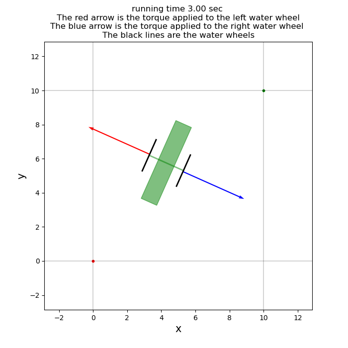
    message = (f'running time {t:.2f} sec \n The red arrow is the torque ' +
        f'applied to the left water wheel \n' +
        f'The blue arrow is the torque applied to the right water wheel \n' +
        f'The black lines are the water wheels')
    ax.set_title(message, fontsize=12)

    coords = coords_lam(*state_sol(t), *input_sol(t), *pL_vals)
    line1.set_data([coords[0, 1], coords[0, 2]], [coords[1, 1], coords[1, 2]])
    line2.set_data([coords[0, 3], coords[0, 4]], [coords[1, 3], coords[1, 4]])
    line3.set_data([coords[0, 5], coords[0, 6]], [coords[1, 5], coords[1, 6]])

    boat.set_xy((state_sol(t)[1]-par_map[bS]/2, state_sol(t)[2]-par_map[aS]/2))
    boat.set_angle(np.rad2deg(state_sol(t)[0]))

    pfeil1.set_offsets([coords[0, -4], coords[1, -4]])
    pfeil1.set_UVC(coords[0, -2] , coords[1, -2])

    pfeil2.set_offsets([coords[0, -3], coords[1, -3]])
    pfeil2.set_UVC(coords[0, -1], coords[1, -1])

A frame from the animation.

fig, ax, line1, line2, line3, pfeil1, pfeil2, boat = init_plot()

_ = update(3)

Create the animation.

fig, ax, line1, line2, line3, pfeil1, pfeil2, boat = init_plot()
animation = FuncAnimation(fig, update, frames=np.arange(t0,
    num_nodes*h_val, 1 / fps), interval=1000/fps)

plt.show()

Once Loop Reflect