Note
Go to the end to download the full example code.
Drone Flight
Objectives
Show how to add extra algebraic contraints (in this case, the quaternion magnitude).
Demonstrate automatically generating a linear initial guess between instance constraints.
Introduction
Given a cuboid shaped drone of dimensions l x w x d with propellers at each corner in a uniform gravitational field, find the propeller thrust trajectories that will take it from a starting point to an ending point and through and intermediate point at a specific angular configuration with minimal total thrust.
Constants
m : drone mass, [kg]
l : length (along body x) [m]
w : width (along body y) [m]
d : depth (along body z) [m]
c : viscous friction coefficient of air [Nms]
States
x, y, z : position of mass center [m]
v1, v2, v3 : body fixed speed of mass center [m]
q0, q1, q2, q3 : quaternion measure numbers [rad]
wx, wy, wz: body fixed angular rates [rad/s]
Specifieds
F1, F2, F3, F4 : propeller propulsion forces [N]
import sympy as sm
import sympy.physics.mechanics as me
import numpy as np
from opty import Problem, create_objective_function
import matplotlib.pyplot as plt
import matplotlib.animation as animation
Generate the equations of motion of the system.
m, l, w, d, g, c = sm.symbols('m, l, w, d, g, c', real=True)
x, y, z, vx, vy, vz = me.dynamicsymbols('x, y, z, v_x, v_y v_z', real=True)
q0, q1, q2, q3 = me.dynamicsymbols('q0, q1, q2, q3', real=True)
u0, wx, wy, wz = me.dynamicsymbols('u0, omega_x, omega_y, omega_z', real=True)
F1, F2, F3, F4 = me.dynamicsymbols('F1, F2, F3, F4', real=True)
t = me.dynamicsymbols._t
O, Ao, P1, P2, P3, P4 = sm.symbols('O, A_o, P1, P2, P3, P4', cls=me.Point)
N, A = sm.symbols('N, A', cls=me.ReferenceFrame)
A.orient_quaternion(N, (q0, q1, q2, q3))
Ao.set_pos(O, x*N.x + y*N.y + z*N.z)
P1.set_pos(Ao, l/2*A.x + w/2*A.y)
P2.set_pos(Ao, -l/2*A.x + w/2*A.y)
P3.set_pos(Ao, l/2*A.x - w/2*A.y)
P4.set_pos(Ao, -l/2*A.x - w/2*A.y)
N_w_A = A.ang_vel_in(N)
N_v_P = Ao.pos_from(O).dt(N)
kinematical = sm.Matrix([
vx - N_v_P.dot(A.x),
vy - N_v_P.dot(A.y),
vz - N_v_P.dot(A.z),
u0 - q0.diff(t),
wx - N_w_A.dot(A.x),
wy - N_w_A.dot(A.y),
wz - N_w_A.dot(A.z),
])
A.set_ang_vel(N, wx*A.x + wy*A.y + wz*A.z)
O.set_vel(N, 0)
Ao.set_vel(N, vx*A.x + vy*A.y + vz*A.z)
P1.v2pt_theory(Ao, N, A)
P2.v2pt_theory(Ao, N, A)
P3.v2pt_theory(Ao, N, A)
P4.v2pt_theory(Ao, N, A)
# x: l, y: w, z: d
IA = me.inertia(A, m*(w**2 + d**2)/12, m*(l**2 + d**2)/12, m*(l**2 + w**2)/12)
drone = me.RigidBody('A', Ao, A, m, (IA, Ao))
prop1 = (P1, F1*A.z)
prop2 = (P2, F2*A.z)
prop3 = (P3, F3*A.z)
prop4 = (P4, F4*A.z)
# use a linear simplification of air drag for continuous derivatives
grav = (Ao, -m*g*N.z - c*Ao.vel(N))
# enforce the unit quaternion
holonomic = sm.Matrix([q0**2 + q1**2 + q2**2 + q3**2 - 1])
kane = me.KanesMethod(
N,
(x, y, z, q1, q2, q3),
(vx, vy, vz, wx, wy, wz),
kd_eqs=kinematical,
q_dependent=(q0,),
u_dependent=(u0,),
configuration_constraints=holonomic,
velocity_constraints=holonomic.diff(t),
)
fr, frstar = kane.kanes_equations([drone], [prop1, prop2, prop3, prop4, grav])
eom = kinematical.col_join(fr + frstar).col_join(holonomic)
sm.pprint(eom)
⎡ d ↪
⎢- (-2⋅q₀(t)⋅q₂(t) + 2⋅q₁(t)⋅q₃(t))⋅──(z(t)) - (2⋅q₀(t)⋅q₃(t) + 2⋅q₁(t)⋅q₂(t)) ↪
⎢ dt ↪
⎢ ↪
⎢ d ↪
⎢- (2⋅q₀(t)⋅q₁(t) + 2⋅q₂(t)⋅q₃(t))⋅──(z(t)) - (-2⋅q₀(t)⋅q₃(t) + 2⋅q₁(t)⋅q₂(t)) ↪
⎢ dt ↪
⎢ ↪
⎢ d ↪
⎢- (-2⋅q₀(t)⋅q₁(t) + 2⋅q₂(t)⋅q₃(t))⋅──(y(t)) - (2⋅q₀(t)⋅q₂(t) + 2⋅q₁(t)⋅q₃(t)) ↪
⎢ dt ↪
⎢ ↪
⎢ d ↪
⎢ u₀(t) - ──(q₀(t ↪
⎢ dt ↪
⎢ ↪
⎢ d d ↪
⎢ ωₓ(t) - 2⋅q₀(t)⋅──(q₁(t)) + 2⋅q₁(t)⋅──(q₀(t)) + 2 ↪
⎢ dt dt ↪
⎢ ↪
⎢ d d ↪
⎢ ω_y(t) - 2⋅q₀(t)⋅──(q₂(t)) - 2⋅q₁(t)⋅──(q₃(t)) + ↪
⎢ dt dt ↪
⎢ ↪
⎢ d d ↪
⎢ ω_z(t) - 2⋅q₀(t)⋅──(q₃(t)) + 2⋅q₁(t)⋅──(q₂(t)) - ↪
⎢ dt dt ↪
⎢ ↪
⎢ ↪
⎢ -c⋅vₓ(t) - g⋅m⋅(-2⋅q₀(t)⋅q₂(t) + 2⋅q₁(t)⋅q₃(t)) - m⋅(ω_ ↪
⎢ ↪
⎢ ↪
⎢ ↪
⎢ -c⋅v_y(t) - g⋅m⋅(2⋅q₀(t)⋅q₁(t) + 2⋅q₂(t)⋅q₃(t)) - m⋅(-ω ↪
⎢ ↪
⎢ ↪
⎢ ⎛ 2 2 2 2 ⎞ ↪
⎢ -c⋅v_z(t) - g⋅m⋅⎝q₀ (t) - q₁ (t) - q₂ (t) + q₃ (t)⎠ - m⋅(ωₓ(t)⋅v_y(t) - ↪
⎢ ↪
⎢ ↪
⎢ ⎛ 2 2⎞ d ↪
⎢ ⎛ 2 2⎞ m⋅⎝d + w ⎠⋅──(ωₓ(t)) ⎛ 2 2⎞ ↪
⎢ m⋅⎝d + l ⎠⋅ω_y(t)⋅ω_z(t) dt m⋅⎝l + w ⎠⋅ω ↪
⎢ ───────────────────────── - ───────────────────── - ───────────── ↪
⎢ 12 12 12 ↪
⎢ ↪
⎢ ⎛ 2 2⎞ d ↪
⎢ m⋅⎝d + l ⎠⋅──(ω_y(t)) ↪
⎢ l⋅F₁(t) l⋅F₂(t) l⋅F₃(t) l⋅F₄(t) dt ↪
⎢ - ─────── + ─────── - ─────── + ─────── - ────────────────────── ↪
⎢ 2 2 2 2 12 ↪
⎢ ↪
⎢ ↪
⎢ ⎛ 2 2⎞ ⎛ 2 2⎞ ↪
⎢ m⋅⎝d + l ⎠⋅ωₓ(t)⋅ω_y(t) m⋅⎝d + w ⎠⋅ωₓ(t ↪
⎢ - ──────────────────────── + ──────────────── ↪
⎢ 12 12 ↪
⎢ ↪
⎢ 2 2 2 ↪
⎣ q₀ (t) + q₁ (t) + q₂ (t) ↪
↪ d ⎛ 2 2 2 2 ⎞ d ⎤
↪ ⋅──(y(t)) - ⎝q₀ (t) + q₁ (t) - q₂ (t) - q₃ (t)⎠⋅──(x(t)) + vₓ(t) ⎥
↪ dt dt ⎥
↪ ⎥
↪ d ⎛ 2 2 2 2 ⎞ d ⎥
↪ ⋅──(x(t)) - ⎝q₀ (t) - q₁ (t) + q₂ (t) - q₃ (t)⎠⋅──(y(t)) + v_y(t)⎥
↪ dt dt ⎥
↪ ⎥
↪ d ⎛ 2 2 2 2 ⎞ d ⎥
↪ ⋅──(x(t)) - ⎝q₀ (t) - q₁ (t) - q₂ (t) + q₃ (t)⎠⋅──(z(t)) + v_z(t)⎥
↪ dt dt ⎥
↪ ⎥
↪ ⎥
↪ )) ⎥
↪ ⎥
↪ ⎥
↪ d d ⎥
↪ ⋅q₂(t)⋅──(q₃(t)) - 2⋅q₃(t)⋅──(q₂(t)) ⎥
↪ dt dt ⎥
↪ ⎥
↪ d d ⎥
↪ 2⋅q₂(t)⋅──(q₀(t)) + 2⋅q₃(t)⋅──(q₁(t)) ⎥
↪ dt dt ⎥
↪ ⎥
↪ d d ⎥
↪ 2⋅q₂(t)⋅──(q₁(t)) + 2⋅q₃(t)⋅──(q₀(t)) ⎥
↪ dt dt ⎥
↪ ⎥
↪ d ⎥
↪ y(t)⋅v_z(t) - ω_z(t)⋅v_y(t)) - m⋅──(vₓ(t)) ⎥
↪ dt ⎥
↪ ⎥
↪ d ⎥
↪ ₓ(t)⋅v_z(t) + ω_z(t)⋅vₓ(t)) - m⋅──(v_y(t)) ⎥
↪ dt ⎥
↪ ⎥
↪ d ⎥
↪ ω_y(t)⋅vₓ(t)) - m⋅──(v_z(t)) + F₁(t) + F₂(t) + F₃(t) + F₄(t) ⎥
↪ dt ⎥
↪ ⎥
↪ ⎥
↪ ⎥
↪ _y(t)⋅ω_z(t) w⋅F₁(t) w⋅F₂(t) w⋅F₃(t) w⋅F₄(t) ⎥
↪ ──────────── + ─────── + ─────── - ─────── - ─────── ⎥
↪ 2 2 2 2 ⎥
↪ ⎥
↪ ⎥
↪ ⎛ 2 2⎞ ⎛ 2 2⎞ ⎥
↪ m⋅⎝d + w ⎠⋅ωₓ(t)⋅ω_z(t) m⋅⎝l + w ⎠⋅ωₓ(t)⋅ω_z(t) ⎥
↪ - ──────────────────────── + ──────────────────────── ⎥
↪ 12 12 ⎥
↪ ⎥
↪ ⎛ 2 2⎞ d ⎥
↪ m⋅⎝l + w ⎠⋅──(ω_z(t)) ⎥
↪ )⋅ω_y(t) dt ⎥
↪ ──────── - ────────────────────── ⎥
↪ 12 ⎥
↪ ⎥
↪ 2 ⎥
↪ + q₃ (t) - 1 ⎦
Set up the time discretization.
duration = 10.0 # seconds
num_nodes = 301
interval_value = duration/(num_nodes - 1)
Provide some values for the constants.
par_map = {
c: 0.5*0.1*1.2,
d: 0.1,
g: 9.81,
l: 1.0,
m: 2.0,
w: 0.5,
}
state_symbols = (x, y, z, q0, q1, q2, q3, vx, vy, vz, u0, wx, wy, wz)
specified_symbols = (F1, F2, F3, F4)
Specify the objective function and form the gradient.
obj_func = sm.Integral(F1**2 + F2**2 + F3**2 + F4**2, t)
sm.pprint(obj_func)
obj, obj_grad = create_objective_function(obj_func,
state_symbols,
specified_symbols,
tuple(),
num_nodes,
interval_value,
time_symbol=t)
⌠
⎮ ⎛ 2 2 2 2 ⎞
⎮ ⎝F₁ (t) + F₂ (t) + F₃ (t) + F₄ (t)⎠ dt
⌡
Specify the symbolic instance constraints.
instance_constraints = (
# move from (0, 0, 0) to (10, 10, 10) meters
x.func(0.0),
y.func(0.0),
z.func(0.0),
x.func(duration) - 10.0,
y.func(duration) - 10.0,
z.func(duration) - 10.0,
# start level
q0.func(0.0) - 1.0,
q1.func(0.0),
q2.func(0.0),
q3.func(0.0),
# rotate 90 degrees about x at midpoint in time
q0.func(duration/2) - np.cos(np.pi/4),
q1.func(duration/2) - np.sin(np.pi/4),
q2.func(duration/2),
q3.func(duration/2),
# end level
q0.func(duration) - 1.0,
q1.func(duration),
q2.func(duration),
q3.func(duration),
# stationary at start and finish
vx.func(0.0),
vy.func(0.0),
vz.func(0.0),
u0.func(0.0),
wx.func(0.0),
wy.func(0.0),
wz.func(0.0),
vx.func(duration),
vy.func(duration),
vz.func(duration),
u0.func(duration),
wx.func(duration),
wy.func(duration),
wz.func(duration),
)
Add some physical limits to the propeller thrust.
bounds = {
F1: (-100.0, 100.0),
F2: (-100.0, 100.0),
F3: (-100.0, 100.0),
F4: (-100.0, 100.0),
}
Create the optimization problem and set any options.
prob = Problem(obj, obj_grad, eom, state_symbols,
num_nodes, interval_value,
known_parameter_map=par_map,
instance_constraints=instance_constraints,
bounds=bounds)
prob.add_option('nlp_scaling_method', 'gradient-based')
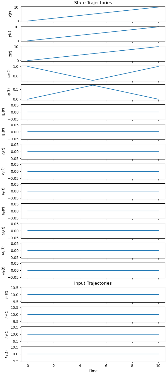
Give a guess of a direct route with constant thrust.
initial_guess = prob.create_linear_initial_guess()
initial_guess[-4*num_nodes:] = 10.0 # constant thrust
fig, axes = plt.subplots(18, 1, sharex=True,
figsize=(6.4, 0.8*18),
layout='compressed')
_ = prob.plot_trajectories(initial_guess, axes=axes)
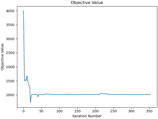
Find an optimal solution.
solution, info = prob.solve(initial_guess)
time = prob.time_vector()
print(info['status_msg'])
print(info['obj_val'])
b'Algorithm terminated successfully at a locally optimal point, satisfying the convergence tolerances (can be specified by options).'
1015.406714782235
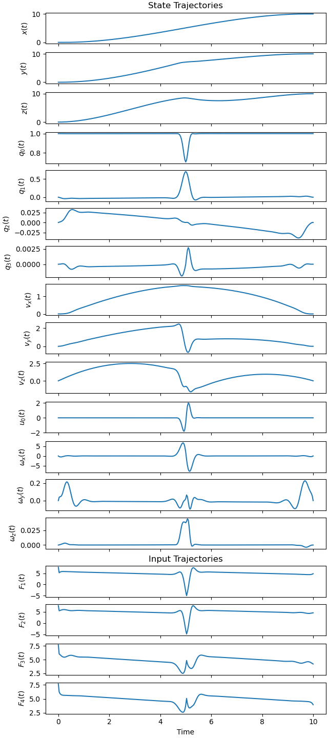
Plot the optimal state and input trajectories.
fig, axes = plt.subplots(18, 1, sharex=True,
figsize=(6.4, 0.8*18),
layout='compressed')
_ = prob.plot_trajectories(solution, axes=axes)
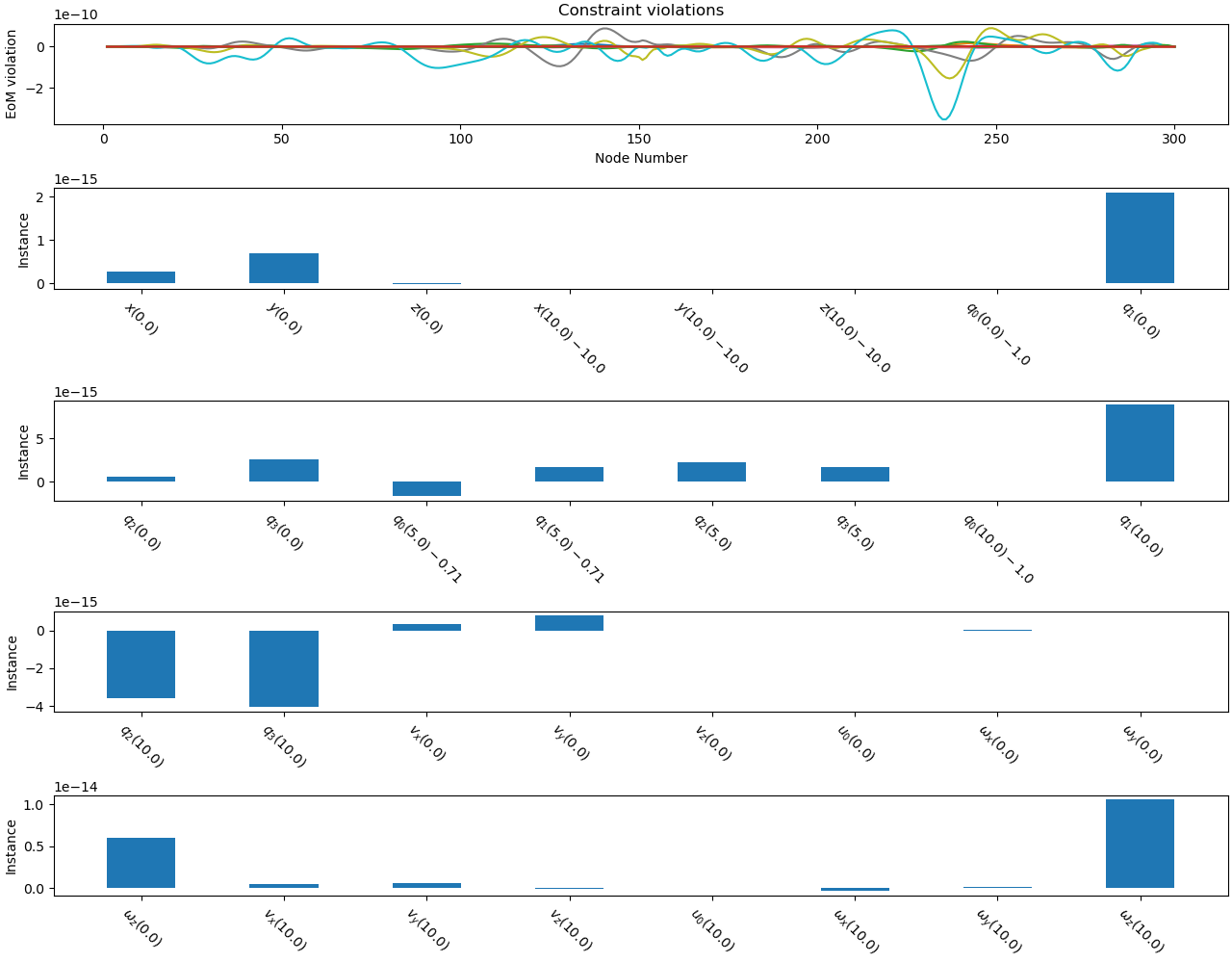
Plot the constraint violations.
fig, axes = plt.subplots(5, 1, figsize=(12.8, 10),
layout='constrained')
_ = prob.plot_constraint_violations(solution, axes=axes)
Plot the objective function as a function of optimizer iteration.
_ = prob.plot_objective_value()
Animate the motion of the drone.
coordinates = Ao.pos_from(O).to_matrix(N)
for point in [P1, Ao, P2, Ao, P3, Ao, P4]:
coordinates = coordinates.row_join(point.pos_from(O).to_matrix(N))
eval_point_coords = sm.lambdify((state_symbols, specified_symbols,
list(par_map.keys())), coordinates, cse=True)
xs, us, ps = prob.parse_free(solution)
coords = []
for xi, ui in zip(xs.T, us.T):
coords.append(eval_point_coords(xi, ui, list(par_map.values())))
coords = np.array(coords) # shape(n, 3, 8)
def frame(i):
fig = plt.figure()
ax = fig.add_subplot(projection='3d')
x, y, z = eval_point_coords(xs[:, i], us[:, i], list(par_map.values()))
drone_lines, = ax.plot(x, y, z,
color='black',
marker='o', markerfacecolor='blue', markersize=4)
P1_path, = ax.plot(coords[:i, 0, 1], coords[:i, 1, 1], coords[:i, 2, 1])
P2_path, = ax.plot(coords[:i, 0, 3], coords[:i, 1, 3], coords[:i, 2, 3])
P3_path, = ax.plot(coords[:i, 0, 5], coords[:i, 1, 5], coords[:i, 2, 5])
P4_path, = ax.plot(coords[:i, 0, 7], coords[:i, 1, 7], coords[:i, 2, 7])
title_template = 'Time = {:1.2f} s'
title_text = ax.set_title(title_template.format(time[i]))
ax.set_xlim((np.min(coords[:, 0, :]) - 0.2,
np.max(coords[:, 0, :]) + 0.2))
ax.set_ylim((np.min(coords[:, 1, :]) - 0.2,
np.max(coords[:, 1, :]) + 0.2))
ax.set_zlim((np.min(coords[:, 2, :]) - 0.2,
np.max(coords[:, 2, :]) + 0.2))
ax.set_xlabel(r'$x$ [m]')
ax.set_ylabel(r'$y$ [m]')
ax.set_zlabel(r'$z$ [m]')
return fig, title_text, drone_lines, P1_path, P2_path, P3_path, P4_path
fig, title_text, drone_lines, P1_path, P2_path, P3_path, P4_path = frame(0)
def animate(i):
title_text.set_text('Time = {:1.2f} s'.format(time[i]))
drone_lines.set_data_3d(coords[i, 0, :], coords[i, 1, :], coords[i, 2, :])
P1_path.set_data_3d(coords[:i, 0, 1], coords[:i, 1, 1], coords[:i, 2, 1])
P2_path.set_data_3d(coords[:i, 0, 3], coords[:i, 1, 3], coords[:i, 2, 3])
P3_path.set_data_3d(coords[:i, 0, 5], coords[:i, 1, 5], coords[:i, 2, 5])
P4_path.set_data_3d(coords[:i, 0, 7], coords[:i, 1, 7], coords[:i, 2, 7])
ani = animation.FuncAnimation(fig, animate, range(0, len(time), 2),
interval=int(interval_value*2000))