Note
Go to the end to download the full example code.
One-Legged Cycling Time Trial

Given a single human leg with four driving lumped muscles powering a fixed gear bicycle and the crank inertia and resistance mimic the torque felt if accelerating the whole bicycle with rider on flat ground, the objective is to travel a specific distance in the shortest amount of time given that the leg muscles have to coordinate.
Warning
This example requires SymPy >= 1.13.
from opty import Problem
from scipy.optimize import fsolve
import matplotlib.animation as animation
import matplotlib.pyplot as plt
import numpy as np
import sympy as sm
import sympy.physics.biomechanics as bm
import sympy.physics.mechanics as me
Coordinates
\(q_1\): crank angle
\(q_2\): pedal angle
\(q_3\): ankle angle
\(q_4\): knee angle
\(u_1\): crank angular rate (cadence)
\(u_2\): pedal angular rate
\(u_3\): ankle angular rate
\(u_4\): knee angular rate
t = me.dynamicsymbols._t
q1, q2, q3, q4 = me.dynamicsymbols('q1, q2, q3, q4', real=True)
u1, u2, u3, u4 = me.dynamicsymbols('u1, u2, u3, u4', real=True)
q = sm.Matrix([q1, q2, q3, q4])
u = sm.Matrix([u1, u2, u3, u4])
qd_repl = {q1.diff(t): u1, q2.diff(t): u2,
           q3.diff(t): u3, q4.diff(t): u4}
Constants
\(l_s\): seat tube length
\(l_c\): crank length
\(l_f\): distance from pedal-foot contact to ankle
\(l_l\): lower leg length
\(l_u\): upper leg length
\(\lambda\): seat tube angle
\(g\): acceleration due to gravity
\(r_k\): knee wrapping radius
\(c\): torsional viscous damping coefficient
\(m_A\): mass of crank
\(m_B\): mass of foot and pedal
\(m_C\): mass of lower leg
\(m_D\): mass of upper leg
\(I_{Azz}\): moment of inertia of crank
\(I_{Bzz}\): moment of inertia of foot and pedal
\(I_{Czz}\): moment of inertia of lower leg
\(I_{Dzz}\): moment of inertia of upper leg
\(J\): rotational moment of inertia of a single bicycle wheel
\(m\): combined mass of the bicycle and cyclist
\(r_w\): wheel radius
\(G\): gear ratio between crank and wheel
\(C_r\): coefficient of rolling resistance
\(C_D\): coefficient of drag
\(\rho\): density of air
\(A_r\): frontal area of bicycle and cyclist
ls, lc, lf, ll, lu = sm.symbols('ls, lc, lf, ll, lu',
                                real=True, positive=True)
lam, g, rk, c = sm.symbols('lam, g, rk, c',
                           real=True, nonnegative=True)
mA, mB, mC, mD = sm.symbols('mA, mB, mC, mD',
                            nonnegative=True)
IAzz, IBzz, ICzz, IDzz = sm.symbols('IAzz, IBzz, ICzz, IDzz',
                                    nonnegative=True)
J, m, rw, G, Cr, CD, rho, Ar = sm.symbols('J, m, rw, G, Cr, CD, rho, Ar',
                                          nonnegative=True)
Reference Frames
\(N\): inertial reference frame for leg dynamics
\(A\): crank
\(B\): foot
\(C\): lower leg
\(D\): upper leg
N, A, B, C, D = sm.symbols('N, A, B, C, D', cls=me.ReferenceFrame)

A.orient_axis(N, N.z, q1)  # crank angle
B.orient_axis(A, A.z, q2)  # pedal angle
C.orient_axis(B, B.z, q3)  # ankle angle
D.orient_axis(C, C.z, q4)  # knee angle

A.set_ang_vel(N, u1*N.z)
B.set_ang_vel(A, u2*A.z)
C.set_ang_vel(B, u3*B.z)
D.set_ang_vel(C, u4*C.z)
Point Kinematics
\(P_1\) : crank center
\(P_2\) : pedal center
\(P_3\) : ankle
\(P_4\) : knee
\(P_5\) : hip
\(P_6\) : seat center
\(P_7\) : heel
\(P_8\) : knee muscle lower leg insertion point
\(P_9\) : ankle muscle lower leg insertion point
\(A_o\) : mass center of the crank
\(B_o\) : mass center of the pedal and foot
\(C_o\) : mass center of the lower leg
\(D_o\) : mass center of the upper leg
P1, P2, P3, P4, P5, P6, P7, P8, P9 = sm.symbols(
    'P1, P2, P3, P4, P5, P6, P7, P8, P9', cls=me.Point)
Ao, Bo, Co, Do = sm.symbols('Ao, Bo, Co, Do', cls=me.Point)

Ao.set_pos(P1, 0*A.x)
P2.set_pos(P1, lc*A.x)  # pedal center
Bo.set_pos(P2, lf/2*B.x)  # foot mass center
P3.set_pos(P2, lf*B.x)  # ankle
P7.set_pos(P2, 3*lf/2*B.x)  # heel

Co.set_pos(P3, ll/2*C.x)  # lower leg mass center
P4.set_pos(P3, ll*C.x)  # knee

Do.set_pos(P4, lu/2*D.x)  # upper leg mass center
P5.set_pos(P4, lu*D.x)  # hip

P6.set_pos(P1, -ls*sm.cos(lam)*N.x + ls*sm.sin(lam)*N.y)  # seat
P8.set_pos(P3, ll/6*C.x)
P9.set_pos(P4, -2*rk*C.x)

P1.set_vel(N, 0)
P6.set_vel(N, 0)
Ao.v2pt_theory(P1, N, A)
P2.v2pt_theory(P1, N, A)
P7.v2pt_theory(P2, N, B)
Bo.v2pt_theory(P2, N, B)
P3.v2pt_theory(P2, N, B)
Co.v2pt_theory(P3, N, C)
P8.v2pt_theory(P3, N, C)
P9.v2pt_theory(P3, N, C)
P4.v2pt_theory(P3, N, C)
Do.v2pt_theory(P4, N, D)
P5.v2pt_theory(P4, N, D)

kindiff = sm.Matrix([ui - qi.diff(t) for ui, qi in zip(u, q)])
Holonomic Constraints
The leg forms a kinematic loop and two holonomic constraints arise from this loop.
holonomic = (P5.pos_from(P1) - P6.pos_from(P1)).to_matrix(N)[:2, :]
mocon = me.msubs(holonomic.diff(t), qd_repl)
sm.trigsimp(mocon)
Matrix([
[-lc*u1(t)*sin(q1(t)) - lf*(u1(t) + u2(t))*sin(q1(t) + q2(t)) - ll*(u1(t) + u2(t) + u3(t))*sin(q1(t) + q2(t) + q3(t)) - lu*(u1(t) + u2(t) + u3(t) + u4(t))*sin(q1(t) + q2(t) + q3(t) + q4(t))],
[ lc*u1(t)*cos(q1(t)) + lf*(u1(t) + u2(t))*cos(q1(t) + q2(t)) + ll*(u1(t) + u2(t) + u3(t))*cos(q1(t) + q2(t) + q3(t)) + lu*(u1(t) + u2(t) + u3(t) + u4(t))*cos(q1(t) + q2(t) + q3(t) + q4(t))]])
Inertia and Rigid Bodies
IA = me.Inertia.from_inertia_scalars(Ao, A, 0, 0, IAzz)
IB = me.Inertia.from_inertia_scalars(Bo, B, 0, 0, IBzz)
IC = me.Inertia.from_inertia_scalars(Co, C, 0, 0, ICzz)
ID = me.Inertia.from_inertia_scalars(Do, D, 0, 0, IDzz)

crank = me.RigidBody('crank', masscenter=Ao, frame=A,
                     mass=mA, inertia=IA)
foot = me.RigidBody('foot', masscenter=Bo, frame=B,
                    mass=mB, inertia=IB)
lower_leg = me.RigidBody('lower leg', masscenter=Co, frame=C,
                         mass=mC, inertia=IC)
upper_leg = me.RigidBody('upper leg', masscenter=Do, frame=D,
                         mass=mD, inertia=ID)
Forces
Gravity acts on each leg body segment.
gravB = me.Force(Bo, -mB*g*N.y)
gravC = me.Force(Co, -mC*g*N.y)
gravD = me.Force(Do, -mD*g*N.y)
Crank Resistance
Model the resistance torque at the crank to be that which one would feel when accelerating the bicycle and cyclist along flat ground. The basic equations of motion of a point mass model of a cyclist are:
where \(T_w\) is the rear wheel driving torque.
The angular speed of the rear wheel is related to the crank cadence by the gear ratio \(G\):
The torque applied to the crank to drive the vehicle is then:
The \(\operatorname{sgn}\) function that manages the sign of the drag force has a discontinuity and is not differentiable. Since we only want to solve this optimal control problem for forward motion we can make the assumption that \(u_1 \leq 0\). The torque felt back on the crank is then:
resistance = me.Torque(
    crank,
    (-(2*J + m*rw**2)*G**2*u1.diff()
     + Cr*m*g*rw*G
     + rho*CD*Ar*G**3*rw**3*u1**2/2)*N.z,
)
Muscles
Lump all the muscles that contribute to joint torques at the knee and ankle into four simplified muscles. The quadriceps wrap over the knee. The other three muscle groups act on linear pathways.
class ExtensorPathway(me.PathwayBase):
    def __init__(self, origin, insertion, axis_point, axis, parent_axis,
                 child_axis, radius, coordinate):
        """A custom pathway that wraps a circular arc around a pin joint.  This
        is intended to be used for extensor muscles. For example, a triceps
        wrapping around the elbow joint to extend the upper arm at the elbow.

        Parameters
        ==========
        origin : Point
            Muscle origin point fixed on the parent body (A).
        insertion : Point
            Muscle insertion point fixed on the child body (B).
        axis_point : Point
            Pin joint location fixed in both the parent and child.
        axis : Vector
            Pin joint rotation axis.
        parent_axis : Vector
            Axis fixed in the parent frame (A) that is directed from the pin
            joint point to the muscle origin point.
        child_axis : Vector
            Axis fixed in the child frame (B) that is directed from the pin
            joint point to the muscle insertion point.
        radius : sympyfiable
            Radius of the arc that the muscle wraps around.
        coordinate : sympfiable function of time
            Joint angle, zero when parent and child frames align. Positive
            rotation about the pin joint axis, B with respect to A.

        Notes
        =====
        Only valid for coordinate >= 0.

        """
        super().__init__(origin, insertion)
        self.origin = origin
        self.insertion = insertion
        self.axis_point = axis_point
        self.axis = axis.normalize()
        self.parent_axis = parent_axis.normalize()
        self.child_axis = child_axis.normalize()
        self.radius = radius
        self.coordinate = coordinate
        self.origin_distance = axis_point.pos_from(origin).magnitude()
        self.insertion_distance = axis_point.pos_from(insertion).magnitude()
        self.origin_angle = sm.asin(self.radius/self.origin_distance)
        self.insertion_angle = sm.asin(self.radius/self.insertion_distance)

    @property
    def length(self):
        """Length of the pathway.
        Length of two fixed length line segments and a changing arc length
        of a circle.
        """
        angle = self.origin_angle + self.coordinate + self.insertion_angle
        arc_length = self.radius*angle
        origin_segment_length = self.origin_distance*sm.cos(self.origin_angle)
        insertion_segment_length = self.insertion_distance*sm.cos(
            self.insertion_angle)
        return origin_segment_length + arc_length + insertion_segment_length

    @property
    def extension_velocity(self):
        """Extension velocity of the pathway.
        Arc length of circle is the only thing that changes when the elbow
        flexes and extends.
        """
        return self.radius*self.coordinate.diff(me.dynamicsymbols._t)

    def to_loads(self, force_magnitude):
        """Loads in the correct format to be supplied to `KanesMethod`.
        Forces applied to origin, insertion, and P from the muscle wrapped
        over circular arc of radius r.
        """
        self.parent_tangency_point = me.Point('Aw')  # fixed in parent
        self.child_tangency_point = me.Point('Bw')  # fixed in child
        self.parent_tangency_point.set_pos(
            self.axis_point,
            -self.radius*sm.cos(self.origin_angle)*self.parent_axis.cross(
                self.axis)
            + self.radius*sm.sin(self.origin_angle)*self.parent_axis,
        )
        self.child_tangency_point.set_pos(
            self.axis_point,
            self.radius*sm.cos(self.insertion_angle)*self.child_axis.cross(
                self.axis)
            + self.radius*sm.sin(self.insertion_angle)*self.child_axis),
        parent_force_direction_vector = self.origin.pos_from(
            self.parent_tangency_point)
        child_force_direction_vector = self.insertion.pos_from(
            self.child_tangency_point)
        force_on_parent = (force_magnitude*
                           parent_force_direction_vector.normalize())
        force_on_child = (force_magnitude*
                          child_force_direction_vector.normalize())
        loads = [
            me.Force(self.origin, force_on_parent),
            me.Force(self.axis_point, -(force_on_parent + force_on_child)),
            me.Force(self.insertion, force_on_child),
        ]
        return loads


knee_top_pathway = ExtensorPathway(P9, P5, P4, C.z, -C.x, D.x, rk, q4)
knee_top_act = bm.FirstOrderActivationDeGroote2016.with_defaults(
    'knee_top')
knee_top_mus = bm.MusculotendonDeGroote2016.with_defaults(
    'knee_top', knee_top_pathway, knee_top_act)
knee_bot_pathway = me.LinearPathway(P9, P5)
knee_bot_act = bm.FirstOrderActivationDeGroote2016.with_defaults(
    'knee_bot')
knee_bot_mus = bm.MusculotendonDeGroote2016.with_defaults(
    'knee_bot', knee_bot_pathway, knee_bot_act)
ankle_top_pathway = me.LinearPathway(P8, P2)
ankle_top_act = bm.FirstOrderActivationDeGroote2016.with_defaults(
    'ankle_top')
ankle_top_mus = bm.MusculotendonDeGroote2016.with_defaults(
    'ankle_top', ankle_top_pathway, ankle_top_act)
ankle_bot_pathway = me.LinearPathway(P8, P7)
ankle_bot_act = bm.FirstOrderActivationDeGroote2016.with_defaults(
    'ankle_bot')
ankle_bot_mus = bm.MusculotendonDeGroote2016.with_defaults(
    'ankle_bot', ankle_bot_pathway, ankle_bot_act)
Joint Viscous Damping
The high stiffness in the ankle joint can be tamed some by adding some viscous damping in the ankle joint.
ankle_damping_B = me.Torque(B, c*u3*B.z)
ankle_damping_C = me.Torque(C, -c*u3*B.z)
Form the Equations of Motion
kane = me.KanesMethod(
    N,
    (q1, q2),
    (u1, u2),
    kd_eqs=kindiff[:],
    q_dependent=(q3, q4),
    configuration_constraints=holonomic,
    velocity_constraints=mocon,
    u_dependent=(u3, u4),
    constraint_solver='CRAMER',
)

bodies = (crank, foot, lower_leg, upper_leg)

loads = (
    knee_top_mus.to_loads() +
    knee_bot_mus.to_loads() +
    ankle_top_mus.to_loads() +
    ankle_bot_mus.to_loads() +
    [ankle_damping_B, ankle_damping_C, resistance,
     gravB, gravC, gravD]
)

Fr, Frs = kane.kanes_equations(bodies, loads)

muscle_diff_eq = sm.Matrix([
    knee_top_mus.a.diff() - knee_top_mus.rhs()[0, 0],
    knee_bot_mus.a.diff() - knee_bot_mus.rhs()[0, 0],
    ankle_top_mus.a.diff() - ankle_top_mus.rhs()[0, 0],
    ankle_bot_mus.a.diff() - ankle_bot_mus.rhs()[0, 0],
])
The full equations of motion in implicit form are made up of the 4 kinematical differential equations, \(\mathbf{f}_k\), the 2 dynamical differential equations, \(\mathbf{f}_d\), the 4 musculo-tendon differential equations, \(\mathbf{f}_a\), and the 2 holonomic constraint equations, \({f}_h\).
eom = kindiff.col_join(
    Fr + Frs).col_join(
    muscle_diff_eq).col_join(
    holonomic)

state_vars = (
    q1, q2, q3, q4, u1, u2, u3, u4,
    knee_top_mus.a,
    knee_bot_mus.a,
    ankle_top_mus.a,
    ankle_bot_mus.a,
)
state_vars
(q1(t), q2(t), q3(t), q4(t), u1(t), u2(t), u3(t), u4(t), a_knee_top(t), a_knee_bot(t), a_ankle_top(t), a_ankle_bot(t))
Objective
The objective is to cycle as fast as possible, so we need to find the minimal time duration for a fixed distance (or more simply crank revolutions). This can be written mathematically as:
This discretizes to:
If \(h\) is constant, then we can simply minimize \(h\). With the objective being \(h\), the gradient of the objective with respect to all of the free optimization variables is zero except for the single entry of \(\frac{\partial h}{\partial h} = 1\).
def obj(free):
    """Return h (always the last element in the free variables)."""
    return free[-1]


def gradient(free):
    """Return the gradient of the objective."""
    grad = np.zeros_like(free)
    grad[-1] = 1.0
    return grad
Define Numerical Constants
par_map = {
    Ar: 0.55,  # m^2, Tab 5.1, pg 188 Wilson 2004, Upright commuting bike
    CD: 1.15,  # unitless, Tab 5.1, pg 188 Wilson 2004, Upright commuting bike
    Cr: 0.006,  # unitless, Tab 5.1, pg 188 Wilson 2004, Upright commuting bike
    G: 2.0,
    IAzz: 0.0,
    IBzz: 0.01,  # guess, TODO
    ICzz: 0.101,  # lower_leg_inertia [kg*m^2]
    IDzz: 0.282,  # upper_leg_inertia [kg*m^2],
    J: 0.1524,  # from Browser Jason's thesis (rear wheel)
    g: 9.81,
    lam: np.deg2rad(75.0),
    lc: 0.175,  # crank length [m]
    lf: 0.08,  # pedal to ankle [m]
    ll: 0.611,  # lower_leg_length [m]
    ls: 0.8,  # seat tube length [m]
    lu: 0.424,  # upper_leg_length [m],
    m: 85.0,  # kg
    # mA: 0.0,  # not in eom
    mB: 1.0,  # foot mass [kg] guess TODO
    mC: 6.769,  # lower_leg_mass [kg]
    mD: 17.01,  # upper_leg_mass [kg],
    rho: 1.204,  # kg/m^3, air density
    rk: 0.04,  # m, knee radius
    rw: 0.3,  # m, wheel radius
    c: 30.0,  # joint viscous damping [Nms]
    ankle_bot_mus.F_M_max: 1000.0,
    ankle_bot_mus.l_M_opt: np.nan,
    ankle_bot_mus.l_T_slack: np.nan,
    ankle_top_mus.F_M_max: 400.0,
    ankle_top_mus.l_M_opt: np.nan,
    ankle_top_mus.l_T_slack: np.nan,
    knee_bot_mus.F_M_max: 1200.0,
    knee_bot_mus.l_M_opt: np.nan,
    knee_bot_mus.l_T_slack: np.nan,
    knee_top_mus.F_M_max: 1400.0,
    knee_top_mus.l_M_opt: np.nan,
    knee_top_mus.l_T_slack: np.nan,
}

p = list(par_map.keys())
p_vals = np.array(list(par_map.values()))
To get estimates of the tendon slack length, align the crank with the seat tube to maximally extend the knee and hold the foot perpendicular to the lower leg then calculate the muscle pathway lengths in this configuration.
q1_ext = -par_map[lam]  # aligned with seat post
q2_ext = 3.0*np.pi/2.0  # foot perpendicular to crank
eval_holonomic = sm.lambdify((q, p), holonomic)
q3_ext, q4_ext = fsolve(lambda x: eval_holonomic([q1_ext, q2_ext, x[0], x[1]],
                                                 p_vals).squeeze(),
                        x0=np.deg2rad([-100.0, 20.0]))
q_ext = np.array([q1_ext, q2_ext, q3_ext, q4_ext])

eval_mus_lens = sm.lambdify((q, p),
                            (ankle_bot_mus.pathway.length.xreplace(qd_repl),
                             ankle_top_mus.pathway.length.xreplace(qd_repl),
                             knee_bot_mus.pathway.length.xreplace(qd_repl),
                             knee_top_mus.pathway.length.xreplace(qd_repl)),
                            cse=True)
akb_len, akt_len, knb_len, knt_len = eval_mus_lens(q_ext, p_vals)
# length of muscle path when fully extended
par_map[ankle_top_mus.l_T_slack] = akt_len/2
par_map[ankle_bot_mus.l_T_slack] = akb_len/2
par_map[knee_top_mus.l_T_slack] = knt_len/2
par_map[knee_bot_mus.l_T_slack] = knb_len/2
par_map[ankle_top_mus.l_M_opt] = akt_len/2 + 0.01
par_map[ankle_bot_mus.l_M_opt] = akb_len/2 + 0.01
par_map[knee_top_mus.l_M_opt] = knt_len/2 + 0.01
par_map[knee_bot_mus.l_M_opt] = knb_len/2 + 0.01

p_vals = np.array(list(par_map.values()))
Plot Extended Configuration
plot_points = [P6, P1, P2, P3, P7, P3, P4, P5]
coordinates = P6.pos_from(P1).to_matrix(N)
for Pi in plot_points[1:]:
    coordinates = coordinates.row_join(Pi.pos_from(P1).to_matrix(N))
eval_coordinates = sm.lambdify((q, p), coordinates)

mus_points = [P7, P8, P2, P8, None, P9, P6,
              knee_top_pathway.child_tangency_point, None,
              knee_top_pathway.parent_tangency_point, P9]
mus_coordinates = P7.pos_from(P1).to_matrix(N)
for Pi in mus_points[1:]:
    if Pi is None:
        pi_coord = sm.Matrix([sm.nan, sm.nan, sm.nan])
    else:
        pi_coord = Pi.pos_from(P1).to_matrix(N)
    mus_coordinates = mus_coordinates.row_join(pi_coord)
eval_mus_coordinates = sm.lambdify((q, p), mus_coordinates)

title_template = 'Time = {:1.2f} s'


def plot_configuration(q_vals, p_vals, ax=None):
    if ax is None:
        fig, ax = plt.subplots(layout='constrained')

    x, y, _ = eval_coordinates(q_vals, p_vals)
    xm, ym, _ = eval_mus_coordinates(q_vals, p_vals)
    crank_circle = plt.Circle((0.0, 0.0), par_map[lc], fill=False,
                              linestyle='--')
    bike_lines, = ax.plot(x[:3], y[:3], 'o-', linewidth=2, color='#3dcfc2ff')
    leg_lines, = ax.plot(x[2:], y[2:], 'o-', linewidth=4, color='#ffd90fff')
    mus_lines, = ax.plot(xm, ym, 'o-', color='#800080ff',)
    knee_circle = plt.Circle((x[6], y[6]), par_map[rk], color='#800080ff',
                             fill=False)
    ax.add_patch(crank_circle)
    ax.add_patch(knee_circle)
    title_text = ax.set_title(title_template.format(0.0))
    ax.set_aspect('equal')
    return ax, fig, bike_lines, leg_lines, mus_lines, knee_circle, title_text


_ = plot_configuration(q_ext, p_vals)
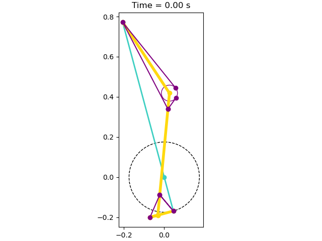
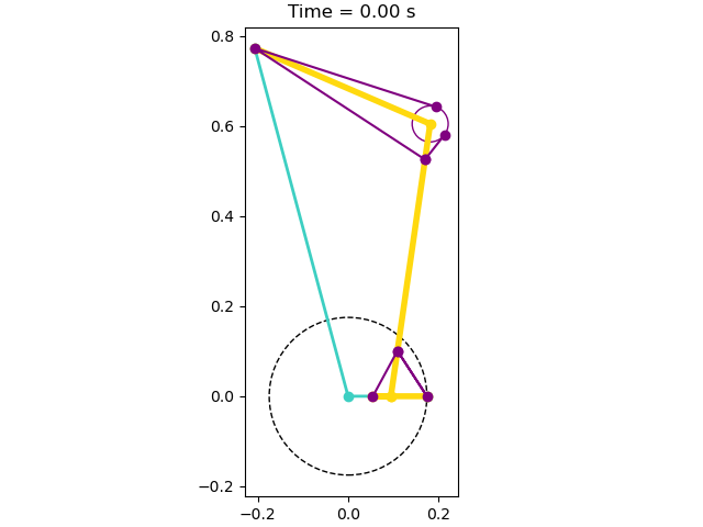
Instance Constraints
The cyclist should start with no motion (stationary) and in an initial configuration with the crank forward and horizontal (\(q_1=0\) deg) and the toe forward and foot parallel to the crank (\(q_2=180\) deg).
q1_0 = 0.0
q2_0 = np.pi
eval_holonomic = sm.lambdify((q, p), holonomic)
q3_0, q4_0 = fsolve(lambda x: eval_holonomic([q1_0, q2_0, x[0], x[1]],
                                             p_vals).squeeze(),
                    x0=np.deg2rad([-90.0, 90.0]), xtol=1e-14)
q_0 = np.array([q1_0, q2_0, q3_0, q4_0])

_ = plot_configuration(q_0, p_vals)
Crank revolutions are proportional to distance traveled so the race distance is defined by number of crank revolutions.
distance = 10.0  # meters
crank_revs = distance/par_map[rw]/par_map[G]/2.0/np.pi  # revolutions
samples_per_rev = 100
num_nodes = int(crank_revs*samples_per_rev)

h = sm.symbols('h', real=True)

instance_constraints = (
    # set the initial configuration
    q1.replace(t, 0*h) - q1_0,
    q2.replace(t, 0*h) - q2_0,
    q3.replace(t, 0*h) - q3_0,
    q4.replace(t, 0*h) - q4_0,
    # start stationary
    u1.replace(t, 0*h),
    u2.replace(t, 0*h),
    u3.replace(t, 0*h),
    u4.replace(t, 0*h),
    # start with no muscle activation
    knee_top_mus.a.replace(t, 0*h),
    knee_bot_mus.a.replace(t, 0*h),
    ankle_top_mus.a.replace(t, 0*h),
    ankle_bot_mus.a.replace(t, 0*h),
    # at final time travel number of revolutions
    q1.replace(t, (num_nodes - 1)*h) + crank_revs*2*np.pi,
)
sm.pprint(instance_constraints)
(q₁(0), q₂(0) - 3.14159265358979, q₃(0) + 1.71407013704151, q₄(0) - 1.30666421 ↪

↪ 361025, u₁(0), u₂(0), u₃(0), u₄(0), aₖₙₑₑ ₜₒₚ(0), a_knee_bot(0), aₐₙₖₗₑ ₜₒₚ( ↪

↪ 0), a_ankle_bot(0), q₁(264⋅h) + 16.6666666666667)
Only allow forward pedaling and limit the joint angle range of motion. All muscle excitations should be bound between 0 and 1.
bounds = {
    q1: (-(crank_revs + 2)*2*np.pi, 0.0),  # can only pedal forward
    # ankle angle, q3=-105 deg: ankle maximally plantar flexed, q3=-30 deg:
    # ankle maximally dorsiflexed
    q3: (-np.deg2rad(105.0), -np.deg2rad(30.)),
    # knee angle, q4 = 0: upper and lower leg aligned, q4 = pi/2: knee is
    # flexed 90 degs
    q4: (0.0, 3*np.pi/2),
    u1: (-30.0, 0.0),  # about 300 rpm
    ankle_bot_mus.e: (0.0, 1.0),
    ankle_top_mus.e: (0.0, 1.0),
    knee_bot_mus.e: (0.0, 1.0),
    knee_top_mus.e: (0.0, 1.0),
    h: (0.0, 0.1),
}
Instantiate the Optimal Control Problem
problem = Problem(
obj,
gradient,
eom,
state_vars,
num_nodes,
h,
known_parameter_map=par_map,
instance_constraints=instance_constraints,
time_symbol=t,
bounds=bounds,
)
problem.add_option('nlp_scaling_method', 'gradient-based')
problem.add_option('max_iter', 1000)
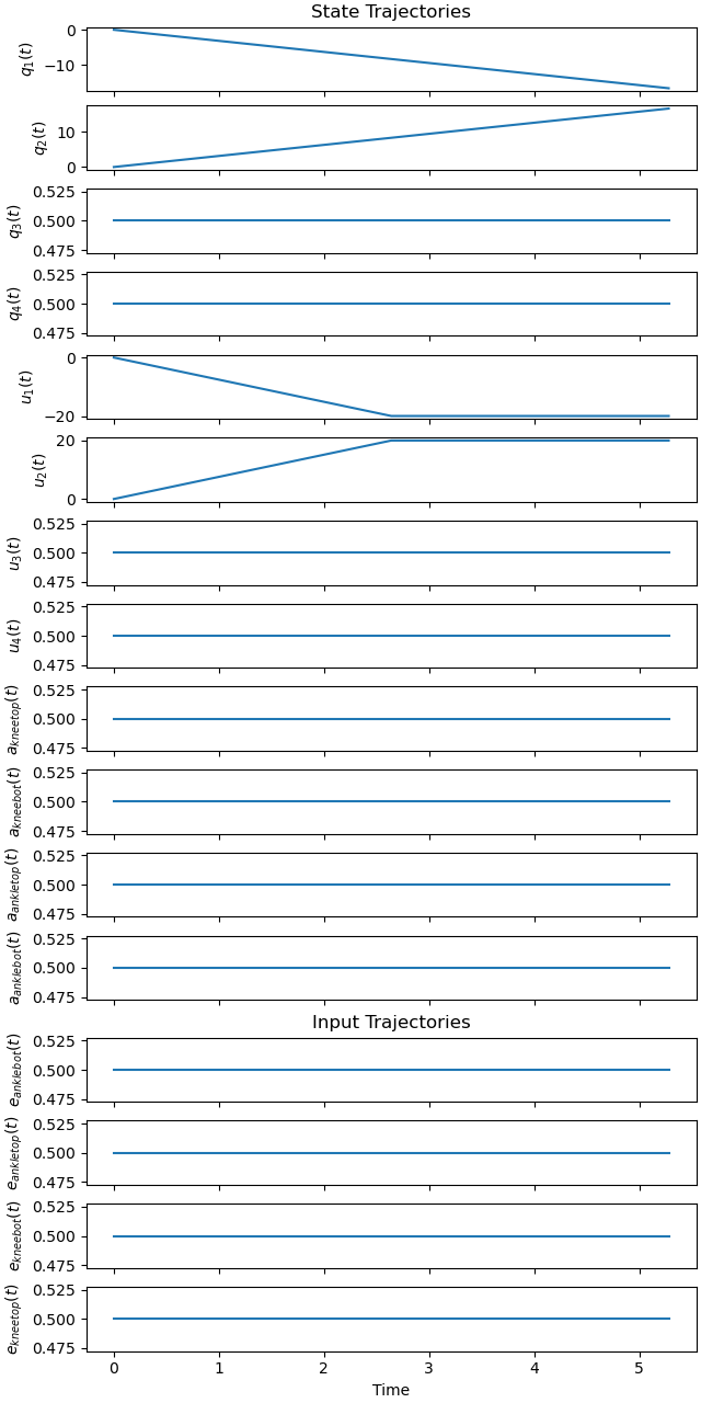
initial_guess = 0.5*np.ones(problem.num_free)
q1_guess = np.linspace(0.0, -crank_revs*2*np.pi, num=num_nodes)
q2_guess = np.linspace(0.0, crank_revs*2*np.pi, num=num_nodes)
u1_guess = np.linspace(0.0, -40.0, num=num_nodes)
u1_guess[num_nodes//2:] = -20.0
u2_guess = np.linspace(0.0, 40.0, num=num_nodes)
u2_guess[num_nodes//2:] = 20.0
initial_guess[0*num_nodes:1*num_nodes] = q1_guess
initial_guess[1*num_nodes:2*num_nodes] = q2_guess
initial_guess[4*num_nodes:5*num_nodes] = u1_guess
initial_guess[5*num_nodes:6*num_nodes] = u2_guess
initial_guess[-1] = 0.02
fig, axes = plt.subplots(16, 1, sharex=True,
figsize=(6.4, 0.8*16),
layout='compressed')
_ = problem.plot_trajectories(initial_guess, axes=axes)
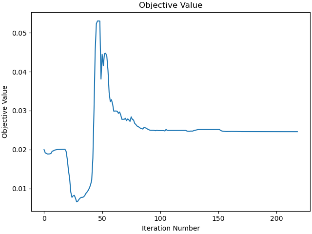
Solve the Optimal Control Problem
solution, info = problem.solve(initial_guess)
xs, us, ps, h_val = problem.parse_free(solution)
print(info['status_msg'])
print('Optimal value h = {:1.3f} s:'.format(h_val))
b'Algorithm terminated successfully at a locally optimal point, satisfying the convergence tolerances (can be specified by options).'
Optimal value h = 0.025 s:
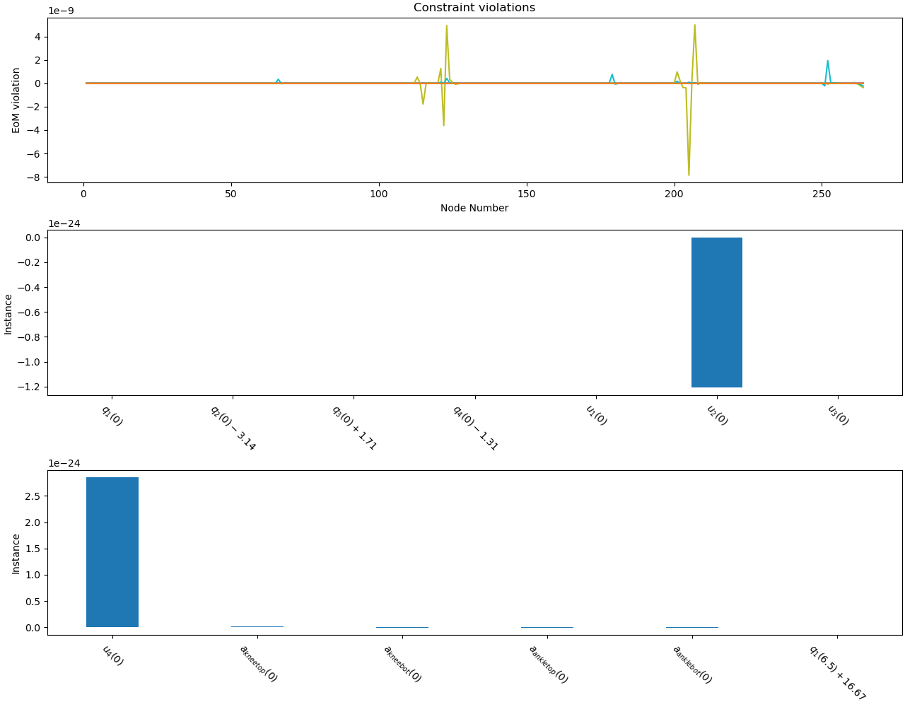
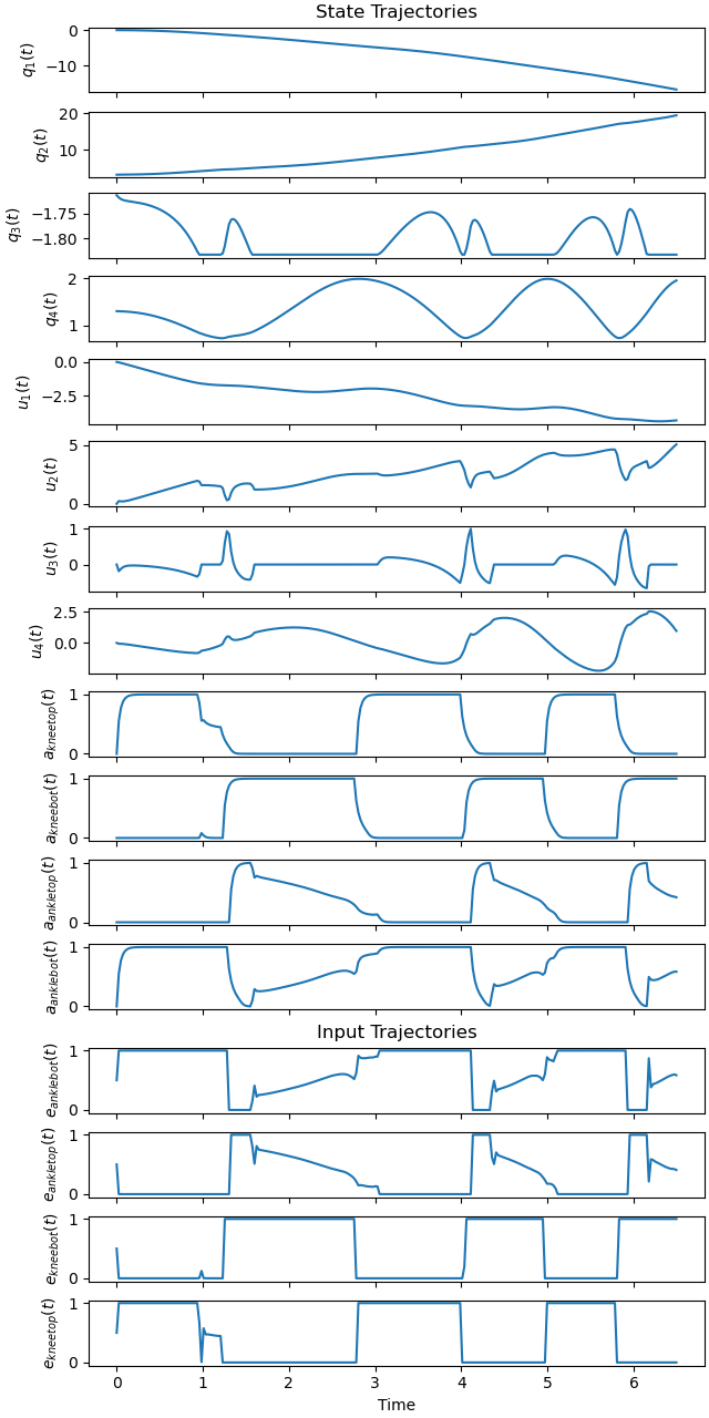
Plot the Solution
_ = problem.plot_objective_value()
fig, axes = plt.subplots(3, 1, figsize=(12.8, 10),
                         layout='constrained')
_ = problem.plot_constraint_violations(solution, axes=axes)
fig, axes = plt.subplots(16, 1, sharex=True,
                         figsize=(6.4, 0.8*16),
                         layout='compressed')
_ = problem.plot_trajectories(solution, axes=axes)
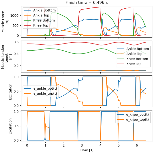
Plot Musculo-tendon Behavior
eval_mus_forces = sm.lambdify(
    (state_vars, p),
    (ankle_bot_mus.force.doit().xreplace(qd_repl),
     ankle_top_mus.force.doit().xreplace(qd_repl),
     knee_bot_mus.force.doit().xreplace(qd_repl),
     knee_top_mus.force.doit().xreplace(qd_repl)),
    cse=True)

akb_for, akt_for, knb_for, knt_for = eval_mus_forces(xs, p_vals)
akb_len, akt_len, knb_len, knt_len = eval_mus_lens(xs[:4], p_vals)


def plot_muscles():

    time = problem.time_vector(solution=solution)

    fig, axes = plt.subplots(4, 1, sharex=True, layout='constrained',
                             figsize=(6.4, 6.4))

    axes[0].set_title('Finish time = {:1.3f} s'.format(time[-1]))
    axes[0].plot(time, -akb_for,
                 time, -akt_for,
                 time, -knb_for,
                 time, -knt_for)
    axes[0].set_ylabel('Muscle Force\n[N]')
    axes[0].legend(['Ankle Bottom', 'Ankle Top',
                    'Knee Bottom', 'Knee Top'])

    axes[1].plot(time, akb_len, time, akt_len,
                 time, knb_len, time, knt_len)
    axes[1].legend(['Ankle Bottom', 'Ankle Top',
                    'Knee Bottom', 'Knee Top'])
    axes[1].set_ylabel('Muscle-tendon\nLength\n[m]')

    axes[2].plot(time, us[0:2, :].T)
    axes[2].legend(problem.collocator.unknown_input_trajectories[0:2])
    axes[2].set_ylabel('Excitation')

    axes[3].plot(time, us[2:4, :].T)
    axes[3].legend(problem.collocator.unknown_input_trajectories[2:4])
    axes[3].set_ylabel('Excitation')

    axes[-1].set_xlabel('Time [s]')

    return axes


_ = plot_muscles()
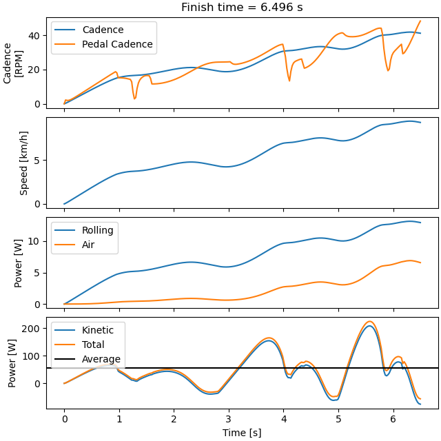
Plot Bike Speed and Rider Power
kin_pow = (2*J + m*rw**2)*G**2*u1.diff()*u1
roll_pow = -Cr*m*g*rw*G*u1
air_pow = -rho*CD*Ar*G**3*rw**3*u1**2/2*u1
eval_pow = sm.lambdify((u1.diff(t), u1, p),
                       (kin_pow, roll_pow, air_pow))
time = problem.time_vector(solution=solution)
u1ds = np.diff(xs[4, :], prepend=0.0)/np.diff(time, prepend=-h_val)
kps, rps, aps = eval_pow(u1ds, xs[4, :], p_vals)


def plot_speed_power():

    fig, axes = plt.subplots(4, 1, sharex=True, layout='constrained',
                             figsize=(6.4, 6.4))

    axes[0].set_title('Finish time = {:1.3f} s'.format(time[-1]))
    axes[0].plot(time, -xs[4, :]*60/2/np.pi,
                 time, xs[5, :]*60/2/np.pi)
    axes[0].set_ylabel('Cadence\n[RPM]')
    axes[0].legend(['Cadence', 'Pedal Cadence'])

    axes[1].plot(time, -xs[4, :]*par_map[G]*par_map[rw]*3.6)
    axes[1].set_ylabel('Speed [km/h]')

    axes[2].plot(time, rps, time, aps)
    axes[2].set_ylabel('Power [W]')
    axes[2].legend(['Rolling', 'Air'])

    axes[3].plot(time, kps,
                 time, kps + rps + aps)
    axes[3].axhline(np.mean(kps + rps + aps), color='black')
    axes[3].set_ylabel('Power [W]')
    axes[3].legend(['Kinetic', 'Total', 'Average'])

    axes[-1].set_xlabel('Time [s]')

    return axes


_ = plot_speed_power()
Animation
ax, fig, bike_lines, leg_lines, mus_lines, knee_circle, title_text = \
    plot_configuration(xs[:4, 0], p_vals)


def animate(i):
    qi = xs[0:4, i]
    x, y, _ = eval_coordinates(qi, p_vals)
    xm, ym, _ = eval_mus_coordinates(qi, p_vals)
    bike_lines.set_data(x[:3], y[:3])
    leg_lines.set_data(x[2:], y[2:])
    mus_lines.set_data(xm, ym)
    knee_circle.set_center((x[6], y[6]))
    title_text.set_text('Time = {:1.2f} s'.format(i*h_val))


ani = animation.FuncAnimation(fig, animate, range(0, num_nodes, 4),
                              interval=int(h_val*4000))

if __name__ == "__main__":
    plt.show()
Total running time of the script: (0 minutes 28.311 seconds)