Note
Go to the end to download the full example code.
Singular Arc Problem
Objective
Show how to optimize a multiphase problem phasewise.
Show how to use a state variable to enforce a boundary condition.
Introduction
This is example 10.47 from [Betts2010], Chapter 10: Test Problems. John T. Betts made available his detailed results of this example, and ‘error’ is the relative error in the value compared to the values given.
This is a three stage problem, where the final state of one stage is the initial state of the next stage.
At the start of phase 2 there is a boundary condition: \(m \cdot g - (1 + \dfrac{v}{c}) \cdot \sigma v^2 e^{-h/h_0} = 0\) It is enforced at the end of phase 1, by introducing a new state variable \(h_\textrm{end}\), and set \(h_{\textrm{end}} = m \cdot g - (1 + \dfrac{v}{c}) \cdot \sigma v^2 e^{-h/h_0}\) and set the instance constraint \(h_{end} = 0\) at the end of phase 1.
Notes
opty presently does not support simultaneous optimization of multiple
phases, so they have to be optimized phasewise.
Dr. Betts confirmed that his solution was achieved by simultaneous
optimization. So, at least in this case, phasewise optimization gives pretty
close results.
Interesting: The last phase, which seems to be the simplest, just free gliding, needs by far the most iterations to converge. Phase 2, the sigular arc, seems to pose no problems at all.
Phase 1 Maximum Thrust
States
\(h, v, m\) : state variables
\(h_{\textrm{end}}\) : state variable to enforce a boundary condition
import numpy as np
import sympy as sm
import sympy.physics.mechanics as me
from opty import Problem
import matplotlib.pyplot as plt
import os
Equations of motion.
t = me.dynamicsymbols._t
h, v, m, h_end = me.dynamicsymbols('h v m, h_end')
h_fast = sm.symbols('h_fast')

# Parameters, the same for all three phases
Tm = 193.044
g = 32.174        # Imperial units
sigma = 5.4915348492 * 1.e-5
c = 1580.942579
h0 = 23800


eom = sm.Matrix([
        -h.diff(t) + v,
        -v.diff(t) + 1/m * (Tm - sigma*v**2*sm.exp(-h/h0)) - g,
        -m.diff(t) - Tm/c,
        -h_end + m*g - (1 + v/c) * sigma*v**2*sm.exp(-h/h0),
])
sm.pprint(eom)
⎡                                          d                                   ↪
⎢                                   v(t) - ──(h(t))                            ↪
⎢                                          dt                                  ↪
⎢                                                                              ↪
⎢                                     -h(t)                                    ↪
⎢                                     ──────                                   ↪
⎢                               2     23800                                    ↪
⎢            - 5.4915348492e-5⋅v (t)⋅ℯ       + 193.044   d                     ↪
⎢            ───────────────────────────────────────── - ──(v(t)) - 32.174     ↪
⎢                              m(t)                      dt                    ↪
⎢                                                                              ↪
⎢                             d                                                ↪
⎢                           - ──(m(t)) - 0.122106901644781                     ↪
⎢                             dt                                               ↪
⎢                                                                              ↪
⎢                                                      -h(t)                   ↪
⎢                                                      ──────                  ↪
⎢                                                2     23800                   ↪
⎣- (3.47358273611277e-8⋅v(t) + 5.4915348492e-5)⋅v (t)⋅ℯ       - h_end(t) + 32. ↪

↪         ⎤
↪         ⎥
↪         ⎥
↪         ⎥
↪         ⎥
↪         ⎥
↪         ⎥
↪         ⎥
↪         ⎥
↪         ⎥
↪         ⎥
↪         ⎥
↪         ⎥
↪         ⎥
↪         ⎥
↪         ⎥
↪         ⎥
↪         ⎥
↪ 174⋅m(t)⎦
num_nodes = 101
t0, tf = 0*h_fast, (num_nodes-1) * h_fast
interval_value = h_fast

state_symbols = (h, v, m, h_end)
Specify the objective function and form the gradient. h(\(t_f\)) is to be maximized. Note that \(h_\textrm{fast}\) is the last entry of free.
def obj(free):
    return -free[num_nodes-1] * free[-1]


def obj_grad(free):
    grad = np.zeros_like(free)
    grad[num_nodes-1] = -free[-1]
    grad[-1] = -free[num_nodes-1]
    return grad


# Specify the symbolic instance constraints, as per the example
instance_constraints = (
        h.func(0*h_fast),
        v.func(0*h_fast),
        m.func(0*h_fast) - 3.0,
        h_end.func(tf),
)

bounds = {
          h_fast: (0.0, 0.5),
          m: (1.0, 3.0)
}
Create the optimization problem and set any options.
prob = Problem(obj,
    obj_grad,
    eom,
    state_symbols,
    num_nodes,
    interval_value,
    instance_constraints=instance_constraints,
    bounds=bounds,
    time_symbol=t,
    backend='numpy',
)

prob.add_option('max_iter', 1000)

# Give some rough estimates for the trajectories.
initial_guess = np.ones(prob.num_free) * 0.1
Find the optimal solution.
solution, info = prob.solve(initial_guess)
print(info['status_msg'])
t_phase1 = solution[-1]
solution1 = solution
b'Algorithm terminated successfully at a locally optimal point, satisfying the convergence tolerances (can be specified by options).'
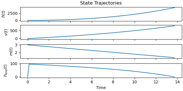
Plot the optimal state and input trajectories.
_ = prob.plot_trajectories(solution)
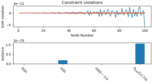
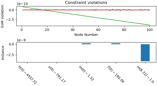
Plot the constraint violations.
_ = prob.plot_constraint_violations(solution)
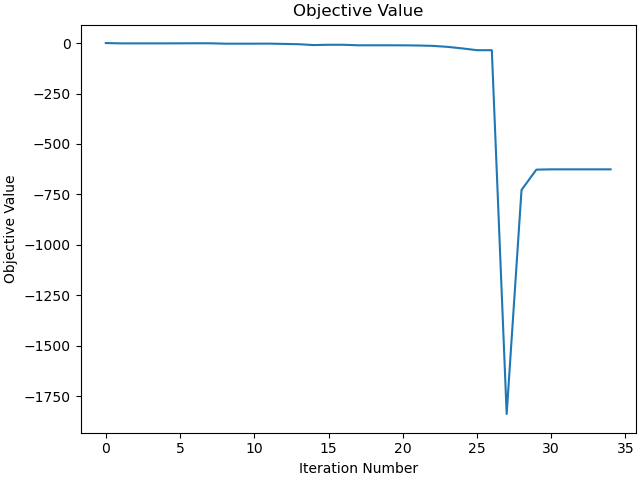
Plot the objective function as a function of optimizer iteration.
prob.plot_objective_value()
error_t = (t_phase1*(num_nodes-1) - 13.726485)/13.726485 * 100
error_v = (solution[2*num_nodes-1] - 791.2744)/791.2744 * 100
error_h = (solution[num_nodes-1] - 4560.8912)/4560.8912 * 100
error_m = (solution[3*num_nodes-1] - 1.323901)/1.323901 * 100
print((f"duration of phase 1 is {(num_nodes-1) * solution[-1]:.3f}, "
       f"error is   {error_t:.3f} %"))
print((f"Height achieved is {- info['obj_val']/solution[-1]:.3f}, "
       f"error is    {error_h:.3f} %"))
print((f"Velocity achieved is {solution[2*num_nodes-1]:.3f}, "
       f"error is   {error_v:.3f} %"))
print(f"Final mass is {solution[3*num_nodes-1]:.3f}, ")
duration of phase 1 is 13.729, error is   0.015 %
Height achieved is 4557.723, error is    -0.069 %
Velocity achieved is 791.166, error is   -0.014 %
Final mass is 1.324,
Phase 2 Singular Arc
Now the thrust T(t) becomes a state variable.
States
\(h, v, m, T\): state variables
# Set up the eoms
T = me.dynamicsymbols('T')


eom = sm.Matrix([
        -h.diff(t) + v,
        -v.diff(t) + 1/m * (T - sigma*v**2*sm.exp(-h/h0)) - g,
        -m.diff(t) - T/c,
        (T - sigma*v**2*sm.exp(-h/h0) - m*g
        -m*g / (1 + 4*c/v + 2*c**2/v**2) * (c**2 / (h0 * g)
                        * (1 + v/c) - 1 - 2 * c/v)),
])

sm.pprint(eom)

state_symbols = (h, v, m, T)
⎡                                                             d                ↪
⎢                                                      v(t) - ──(h(t))         ↪
⎢                                                             dt               ↪
⎢                                                                              ↪
⎢                                                                -h(t)         ↪
⎢                                                                ──────        ↪
⎢                                                          2     23800         ↪
⎢                                  T(t) - 5.4915348492e-5⋅v (t)⋅ℯ         d    ↪
⎢                                  ──────────────────────────────────── - ──(v ↪
⎢                                                  m(t)                   dt   ↪
⎢                                                                              ↪
⎢                                                                        d     ↪
⎢                                           -0.000632534042212042⋅T(t) - ──(m( ↪
⎢                                                                        dt    ↪
⎢                                                                              ↪
⎢                                            -h(t)           ⎛                 ↪
⎢                                            ──────   32.174⋅⎜0.00206459124701 ↪
⎢                                      2     23800           ⎝                 ↪
⎢T(t) - 32.174⋅m(t) - 5.4915348492e-5⋅v (t)⋅ℯ       - ──────────────────────── ↪
⎢                                                                           63 ↪
⎢                                                                       1 + ── ↪
⎢                                                                              ↪
⎣                                                                              ↪

↪                                                ⎤
↪                                                ⎥
↪                                                ⎥
↪                                                ⎥
↪                                                ⎥
↪                                                ⎥
↪                                                ⎥
↪                                                ⎥
↪ (t)) - 32.174                                  ⎥
↪                                                ⎥
↪                                                ⎥
↪                                                ⎥
↪ t))                                            ⎥
↪                                                ⎥
↪                                                ⎥
↪                               3161.885158⎞     ⎥
↪ 662⋅v(t) + 2.26400021063928 - ───────────⎟⋅m(t)⎥
↪                                  v(t)    ⎠     ⎥
↪ ───────────────────────────────────────────────⎥
↪ 23.770316   4998758.87619034                   ⎥
↪ ───────── + ────────────────                   ⎥
↪  v(t)             2                            ⎥
↪                  v (t)                         ⎦
The instance constraints (of course) are the values achieved at the end of the first phase.
instance_constraints = (
        h.func(0*h_fast) - solution[num_nodes-1],
        v.func(0*h_fast) - solution[2*num_nodes-1],
        m.func(0*h_fast) - solution[3*num_nodes-1],
        T.func(0*h_fast) - Tm,
        m.func((num_nodes-1)*h_fast) - 1.0,
)

# As per the example, the mass m >= 1.0
bounds = {
        h_fast: (0.0, 0.5),
        T: (0.0, Tm),
        m: (1.0, solution[3*num_nodes-1])
}
Create the optimization problem and set any options.
prob = Problem(obj,
    obj_grad,
    eom,
    state_symbols,
    num_nodes,
    interval_value,
    instance_constraints=instance_constraints,
    bounds=bounds,
    time_symbol=t,
    backend='numpy',
)

prob.add_option('max_iter', 3000)

# Give some rough estimates for the trajectories.
# The result of a previous run are used to save time.
initial_guess = np.array((*[solution[num_nodes-1] for _ in range(num_nodes)],
                          *[solution[2*num_nodes-1] for _ in range(num_nodes)],
                          *[solution[3*num_nodes-1] for _ in range(num_nodes)],
                          *[Tm/c for _ in range(num_nodes)], solution[-1]))
Find the optimal solution.
solution, info = prob.solve(initial_guess)
initial_guess = solution
print(info['status_msg'])
t_phase2 = solution[-1]
solution2 = solution
b'Algorithm terminated successfully at a locally optimal point, satisfying the convergence tolerances (can be specified by options).'
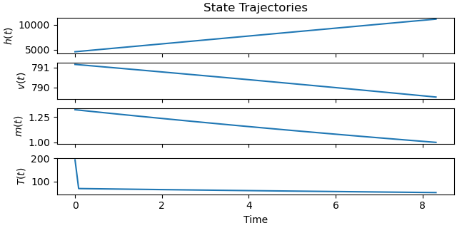
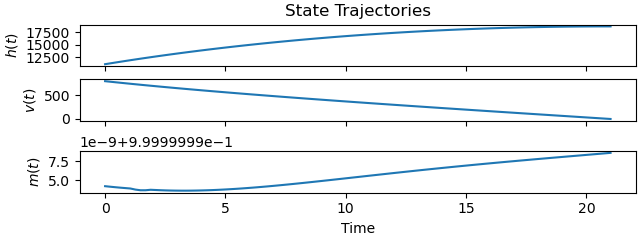
Plot the optimal state and input trajectories.
_ = prob.plot_trajectories(solution)
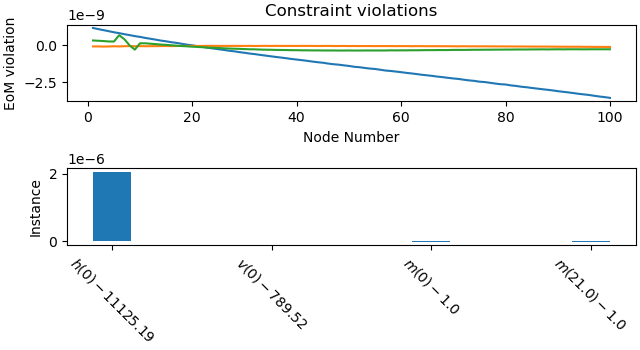
Plot the constraint violations.
_ = prob.plot_constraint_violations(solution)
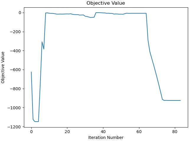
Plot the objective function as a function of optimizer iteration.
_ = prob.plot_objective_value()

error_t = ((t_phase2*(num_nodes-1) - (22.025604-13.726485)) /
           (22.025604-13.726485) * 100)
error_v = (solution[2*num_nodes-1] - 789.64098)/789.64098 * 100
error_h = (solution[num_nodes-1] - 11121.110)/11121.110 * 100
error_m = (solution[3*num_nodes-1] - 1.0)/1.0 * 100
print((f'duration of phase 2 is {(num_nodes-1) * solution[-1]:.3f}, '
       f'error is   {error_t:.3f} %'))
print((f"Height achieved is {- info['obj_val']/solution[-1]:.3f}, "
       f'error is   {error_h:.3f} %'))
print((f'Velocity achieved is {solution[2*num_nodes-1]:.3f}, '
       f'error is  {error_v:.3f} %'))
print(f'Final mass is {solution[3*num_nodes-1]:.3f}, ')
duration of phase 2 is 8.310, error is   0.126 %
Height achieved is 11125.188, error is   0.037 %
Velocity achieved is 789.517, error is  -0.016 %
Final mass is 1.000,
Phase 3 No Thrust
Now it is free gliding without thrust.
States
\(h, v, m\): state variables.
Set up the eoms.
eom = sm.Matrix([
        -h.diff(t) + v,
        -v.diff(t) - sigma*v**2*sm.exp(-h/h0)/m - g,
        -m.diff(t) - 0,
])
sm.pprint(eom)

state_symbols = (h, v, m)
⎡                         d                         ⎤
⎢                  v(t) - ──(h(t))                  ⎥
⎢                         dt                        ⎥
⎢                                                   ⎥
⎢                                             -h(t) ⎥
⎢                                             ──────⎥
⎢                                       2     23800 ⎥
⎢  d                   5.4915348492e-5⋅v (t)⋅ℯ      ⎥
⎢- ──(v(t)) - 32.174 - ─────────────────────────────⎥
⎢  dt                              m(t)             ⎥
⎢                                                   ⎥
⎢                      d                            ⎥
⎢                     -──(m(t))                     ⎥
⎣                      dt                           ⎦
The maximum height is achieved when the velocity is zero. The objective function to be minimized is the square of the final speed. There is really nothing here to be optimized, just stopp when the velocity is zero. However, the ‘obvious’ choice of setting an instance constraint v(\(t_f\)) = 0.0 creates an error message: Problem has too few degrees of freedom.
def obj(free):
    return free[2*num_nodes-1]**2


def obj_grad(free):
    grad = np.zeros_like(free)
    grad[2*num_nodes-1] = 2*free[2*num_nodes-1]
    grad[-1] = 0.0
    return grad


# Specify the symbolic instance constraints. The starting values are the final
# values of the previous phase. The mass must be 1.0 at the end.
instance_constraints = (
        h.func(0*h_fast) - solution[num_nodes-1],
        v.func(0*h_fast) - solution[2*num_nodes-1],
        m.func(0*h_fast) - solution[3*num_nodes-1],
        m.func((num_nodes-1)*h_fast) - 1.0,
)

bounds = {
        h_fast: (0.0, 0.5),
        m: (solution[3*num_nodes-1], 1.0),
        v: (0.0, np.inf),
}
Create the optimization problem and set any options.
prob = Problem(obj,
    obj_grad,
    eom,
    state_symbols,
    num_nodes,
    interval_value,
    instance_constraints=instance_constraints,
    bounds=bounds,
    time_symbol=t,
    backend='numpy',
)

prob.add_option('max_iter', 20000)
fname = f'betts_10_47_phase3_{num_nodes}_nodes_solution.csv'
# Use a given solution if available, else give an initial guess and solve the
# problem.
if os.path.exists(fname):
    solution = np.loadtxt(fname)
    # Use solution given.
    solution = np.loadtxt(fname)
else:
    # Give some rough estimates for the trajectories.
    initial_guess = np.array((*[solution[num_nodes-1] for _ in
                        range(num_nodes)],
                        *[solution[2*num_nodes-1] for _ in range(num_nodes)],
                        *[solution[3*num_nodes-1] for _ in range(num_nodes)],
                        solution[-1])
    )

    # Find the optimal solution.
    solution, info = prob.solve(initial_guess)
    print(info['status_msg'])

    # Plot the objective function as a function of optimizer iteration.
    _ = prob.plot_objective_value()
t_phase3 = solution[-1]
solution3 = solution
# np.savetxt(fname, solution, fmt='%.12f')
Plot the optimal state and input trajectories.
_ = prob.plot_trajectories(solution)
Plot the constraint violations.
_ = prob.plot_constraint_violations(solution)

print(f'final speed is  {solution[2*num_nodes-1]:.3e}, ideally it should be 0')
print('\n')
error_h = (solution[num_nodes-1] - 18664.187)/18664.187 * 100
print((f'final height achieved is is {solution[num_nodes-1]:.3f}, error is '
       f'           {error_h:.3f} %'))

error_t1 = (t_phase1*(num_nodes-1) - 13.751270)/13.751270 * 100
error_t2 = ((t_phase1+t_phase2)*(num_nodes-1) - 21.987)/21.987 * 100
print(('duration of first and second phase is '
       f'{(t_phase1+t_phase2)*(num_nodes-1):.3f}, error is      '
       f'{error_t2:.3f} %'))
error_t3 = (((t_phase1+t_phase2+t_phase3)*(num_nodes-1) - 42.641355)/42.641355
             * 100)
print((f'total duration  is {(t_phase1+t_phase2+t_phase3) * (num_nodes-1):.3f}'
       f' sec, error is                     {error_t3:.3f} %'))
final speed is  1.143e-02, ideally it should be 0


final height achieved is is 18661.338, error is            -0.015 %
duration of first and second phase is 22.038, error is      0.232 %
total duration  is 43.041 sec, error is                     0.937 %
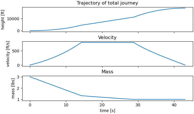
Plot complete journey.
h_list = np.concatenate((solution1[:num_nodes], solution2[:num_nodes],
                        solution3[:num_nodes]))
v_list = np.concatenate((solution1[num_nodes:2*num_nodes],
                        solution2[num_nodes:2*num_nodes],
                        solution3[num_nodes:2*num_nodes]))
m_list = np.concatenate((solution1[2*num_nodes:3*num_nodes],
                        solution2[2*num_nodes:3*num_nodes],
                        solution3[2*num_nodes:3*num_nodes]))

times = np.linspace(0, (num_nodes-1)*(t_phase1+t_phase2+t_phase3), num_nodes*3)
fig, ax = plt.subplots(3, 1, figsize=(6.8, 4), sharex=True,
                       layout='constrained')
ax[0].plot(times, h_list)
ax[0].set_ylabel('height [ft]')
ax[0].set_title('Trajectory of total journey')
ax[1].plot(times, v_list)
ax[1].set_ylabel('velocity [ft/s]')
ax[1].set_title('Velocity')
ax[2].plot(times, m_list)
ax[2].set_ylabel('mass [lbs]')
ax[2].set_xlabel('time [s]')
_ = ax[2].set_title('Mass')
sphinx_gallery_thumbnail_number = 9
Total running time of the script: (0 minutes 7.254 seconds)