Examples
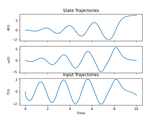
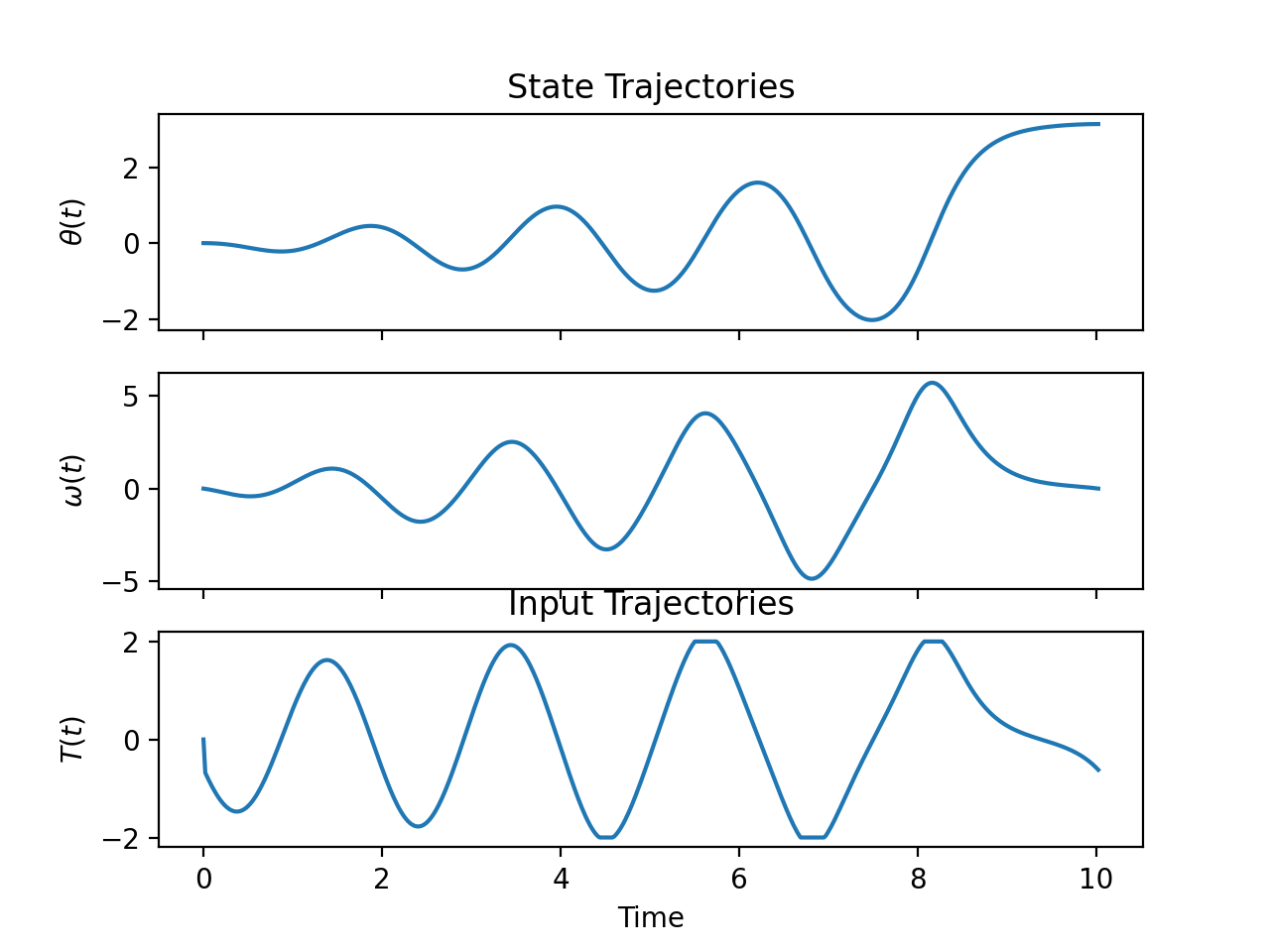
Single Pendulum Swing Up
"""This solves the simple pendulum swing up problem presented here:
http://hmc.csuohio.edu/resources/human-motion-seminar-jan-23-2014
A simple pendulum is controlled by a torque at its joint. The goal is to
swing the pendulum from its rest equilibrium to a target angle by minimizing
the energy used to do so.
"""
from collections import OrderedDict
import numpy as np
import sympy as sym
from opty.direct_collocation import Problem
from opty.utils import building_docs, create_objective_function
import matplotlib.pyplot as plt
import matplotlib.animation as animation
target_angle = np.pi
duration = 10.0
num_nodes = 500
save_animation = False
interval_value = duration / (num_nodes - 1)
# Symbolic equations of motion
I, m, g, d, t = sym.symbols('I, m, g, d, t')
theta, omega, T = sym.symbols('theta, omega, T', cls=sym.Function)
state_symbols = (theta(t), omega(t))
constant_symbols = (I, m, g, d)
specified_symbols = (T(t),)
eom = sym.Matrix([theta(t).diff() - omega(t),
I * omega(t).diff() + m * g * d * sym.sin(theta(t)) - T(t)])
# Specify the known system parameters.
par_map = OrderedDict()
par_map[I] = 1.0
par_map[m] = 1.0
par_map[g] = 9.81
par_map[d] = 1.0
# Specify the objective function and it's gradient.
obj_func = sym.Integral(T(t)**2, t)
obj, obj_grad = create_objective_function(obj_func, state_symbols,
specified_symbols, tuple(),
num_nodes,
node_time_interval=interval_value)
# Specify the symbolic instance constraints, i.e. initial and end
# conditions.
instance_constraints = (theta(0.0),
theta(duration) - target_angle,
omega(0.0),
omega(duration))
# Create an optimization problem.
prob = Problem(obj, obj_grad, eom, state_symbols, num_nodes, interval_value,
known_parameter_map=par_map,
instance_constraints=instance_constraints,
bounds={T(t): (-2.0, 2.0)})
# Use a random positive initial guess.
initial_guess = np.random.randn(prob.num_free)
# Find the optimal solution.
solution, info = prob.solve(initial_guess)
# Make some plots
prob.plot_trajectories(solution)
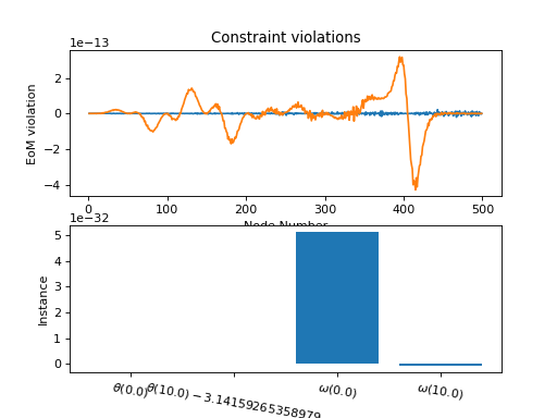
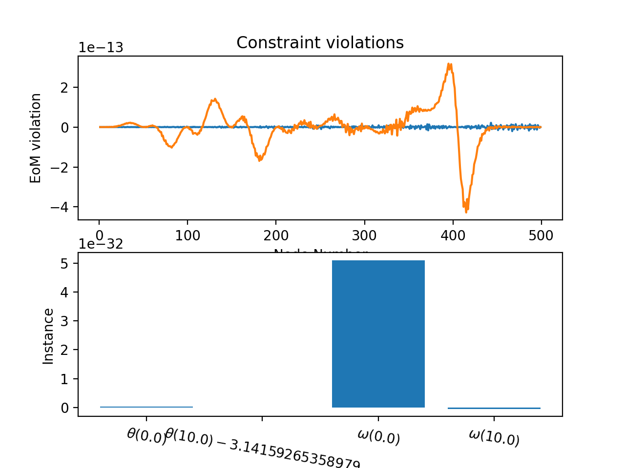
prob.plot_constraint_violations(solution)
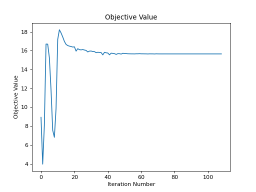
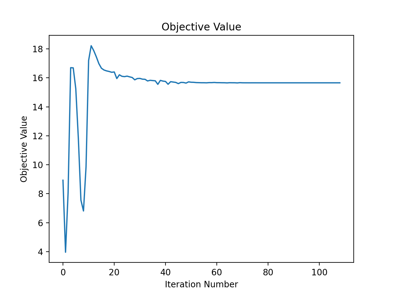
prob.plot_objective_value()
# Display animation
if not building_docs():
time = np.linspace(0.0, duration, num=num_nodes)
angle = solution[:num_nodes]
fig = plt.figure()
ax = fig.add_subplot(111, aspect='equal', autoscale_on=False, xlim=(-2, 2),
ylim=(-2, 2))
ax.grid()
line, = ax.plot([], [], 'o-', lw=2)
time_template = 'time = {:0.1f}s'
time_text = ax.text(0.05, 0.9, '', transform=ax.transAxes)
def init():
line.set_data([], [])
time_text.set_text('')
return line, time_text
def animate(i):
x = [0, par_map[d] * np.sin(angle[i])]
y = [0, -par_map[d] * np.cos(angle[i])]
line.set_data(x, y)
time_text.set_text(time_template.format(i * interval_value))
return line, time_text
ani = animation.FuncAnimation(fig, animate, np.arange(1, len(time)),
interval=25, blit=True, init_func=init)
if save_animation:
ani.save('pendulum_swing_up.mp4', writer='ffmpeg',
fps=1 / interval_value)
plt.show()
Example console output:
******************************************************************************
This program contains Ipopt, a library for large-scale nonlinear optimization.
 Ipopt is released as open source code under the Eclipse Public License (EPL).
         For more information visit http://projects.coin-or.org/Ipopt
******************************************************************************

This is Ipopt version 3.12.8, running with linear solver mumps.
NOTE: Other linear solvers might be more efficient (see Ipopt documentation).

Number of nonzeros in equality constraint Jacobian...:     4994
Number of nonzeros in inequality constraint Jacobian.:        0
Number of nonzeros in Lagrangian Hessian.............:        0

Total number of variables............................:     1500
                     variables with only lower bounds:        0
                variables with lower and upper bounds:      500
                     variables with only upper bounds:        0
Total number of equality constraints.................:     1002
Total number of inequality constraints...............:        0
        inequality constraints with only lower bounds:        0
   inequality constraints with lower and upper bounds:        0
        inequality constraints with only upper bounds:        0

iter    objective    inf_pr   inf_du lg(mu)  ||d||  lg(rg) alpha_du alpha_pr  ls
   0  1.0051250e+01 2.37e+02 8.84e-02   0.0 0.00e+00    -  0.00e+00 0.00e+00   0
   1  3.9969186e+00 1.83e+02 2.29e+01   0.9 8.83e+00    -  6.88e-01 2.29e-01f  1
   2  8.3301435e+00 1.38e+02 4.99e+01  -1.2 8.40e+00    -  3.00e-01 2.53e-01h  1
   3  1.8540696e+01 6.01e+01 5.63e+01  -5.3 6.38e+00    -  4.07e-01 5.70e-01h  1
   4  1.4859148e+01 3.86e+01 1.07e+02   0.7 5.98e+00    -  2.46e-01 3.63e-01f  1
   5  1.2535715e+01 2.48e+01 1.26e+02   0.7 4.54e+00    -  5.28e-01 3.68e-01f  1
   6  1.0337282e+01 2.49e+01 1.53e+02   2.6 1.38e+02    -  5.69e-02 1.96e-02f  1
   7  1.0132779e+01 1.18e+01 5.70e+02   1.4 4.35e+00    -  7.49e-01 5.39e-01h  1
   8  1.0049523e+01 7.13e+00 5.63e+02   1.3 5.26e+00    -  5.52e-01 3.95e-01h  1
   9  1.2555246e+01 4.36e+00 3.29e+02   1.3 4.84e+00    -  6.03e-01 3.96e-01h  1
...
iter    objective    inf_pr   inf_du lg(mu)  ||d||  lg(rg) alpha_du alpha_pr  ls
  80  1.5656141e+01 2.43e-10 2.75e-06 -11.0 4.95e-04    -  1.00e+00 1.00e+00H  1
  81  1.5656141e+01 2.97e-11 1.01e-05 -11.0 3.08e-04    -  1.00e+00 1.00e+00H  1
  82  1.5656141e+01 3.06e-11 2.41e-07 -11.0 2.55e-04    -  1.00e+00 1.00e+00H  1
  83  1.5656141e+01 6.22e-14 3.29e-07 -11.0 1.37e-05    -  1.00e+00 1.00e+00H  1
  84  1.5656141e+01 6.04e-14 5.00e-07 -11.0 4.27e-05    -  1.00e+00 1.00e+00H  1
  85  1.5656141e+01 5.82e-14 4.40e-06 -11.0 9.70e-05    -  1.00e+00 1.00e+00H  1
  86  1.5656141e+01 1.03e-11 3.42e-07 -11.0 9.84e-05    -  1.00e+00 1.00e+00H  1
  87  1.5656141e+01 4.80e-14 3.65e-06 -11.0 1.19e-04    -  1.00e+00 1.00e+00H  1
  88  1.5656141e+01 3.86e-12 2.60e-07 -11.0 1.15e-04    -  1.00e+00 1.00e+00H  1
  89  1.5656141e+01 7.55e-14 1.61e-06 -11.0 4.94e-05    -  1.00e+00 1.00e+00H  1
iter    objective    inf_pr   inf_du lg(mu)  ||d||  lg(rg) alpha_du alpha_pr  ls
  90  1.5656141e+01 6.89e-11 1.67e-08 -11.0 4.29e-05    -  1.00e+00 1.00e+00h  1
  91  1.5656141e+01 4.09e-14 6.37e-09 -11.0 4.51e-07    -  1.00e+00 1.00e+00h  1

Number of Iterations....: 91

                                   (scaled)                 (unscaled)
Objective...............:   1.5656141337135018e+01    1.5656141337135018e+01
Dual infeasibility......:   6.3721938193329774e-09    6.3721938193329774e-09
Constraint violation....:   4.0856207306205761e-14    4.0856207306205761e-14
Complementarity.........:   1.0000001046147741e-11    1.0000001046147741e-11
Overall NLP error.......:   6.3721938193329774e-09    6.3721938193329774e-09


Number of objective function evaluations             = 133
Number of objective gradient evaluations             = 92
Number of equality constraint evaluations            = 133
Number of inequality constraint evaluations          = 0
Number of equality constraint Jacobian evaluations   = 92
Number of inequality constraint Jacobian evaluations = 0
Number of Lagrangian Hessian evaluations             = 0
Total CPU secs in IPOPT (w/o function evaluations)   =      2.756
Total CPU secs in NLP function evaluations           =      0.080

EXIT: Optimal Solution Found.
Betts 2003
"""This is the problem presented in section 7 of:
Betts, John T. and Huffman, William P. "Large Scale Parameter Estimation
Using Sparse Nonlinear Programming Methods". SIAM J. Optim., Vol 14, No. 1,
pp. 223-244, 2003.
"""
from collections import OrderedDict
import numpy as np
import sympy as sym
import matplotlib.pyplot as plt
from opty.direct_collocation import Problem
duration = 1.0
num_nodes = 100
interval = duration / (num_nodes - 1)
# Symbolic equations of motion
mu, p, t = sym.symbols('mu, p, t')
y1, y2, T = sym.symbols('y1, y2, T', cls=sym.Function)
state_symbols = (y1(t), y2(t))
constant_symbols = (mu, p)
# I had to use a little "trick" here because time was explicit in the eoms,
# i.e. setting T(t) to a function of time and then pass in time as a known
# trajectory in the problem.
eom = sym.Matrix([y1(t).diff(t) - y2(t),
y2(t).diff(t) - mu**2 * y1(t) + (mu**2 + p**2) *
sym.sin(p * T(t))])
# Specify the known system parameters.
par_map = OrderedDict()
par_map[mu] = 60.0
# Generate data
time = np.linspace(0.0, 1.0, num_nodes)
y1_m = np.sin(np.pi * time) + np.random.normal(scale=0.05, size=len(time))
y2_m = np.pi * np.cos(np.pi * time) + np.random.normal(scale=0.05,
size=len(time))
# Specify the objective function and it's gradient. I'm only fitting to y1,
# but they may have fit to both states in the paper.
def obj(free):
return interval * np.sum((y1_m - free[:num_nodes])**2)
def obj_grad(free):
grad = np.zeros_like(free)
grad[:num_nodes] = 2.0 * interval * (free[:num_nodes] - y1_m)
return grad
# Specify the symbolic instance constraints, i.e. initial and end
# conditions.
instance_constraints = (y1(0.0), y2(0.0) - np.pi)
# Create an optimization problem.
prob = Problem(obj, obj_grad,
eom, state_symbols,
num_nodes, interval,
known_parameter_map=par_map,
known_trajectory_map={T(t): time},
instance_constraints=instance_constraints,
integration_method='midpoint')
# Use a random positive initial guess.
initial_guess = np.random.randn(prob.num_free)
# Find the optimal solution.
solution, info = prob.solve(initial_guess)
known_msg = "Known value of p = {}".format(np.pi)
identified_msg = "Identified value of p = {}".format(solution[-1])
divider = '=' * max(len(known_msg), len(identified_msg))
print(divider)
print(known_msg)
print(identified_msg)
print(divider)
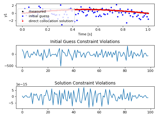
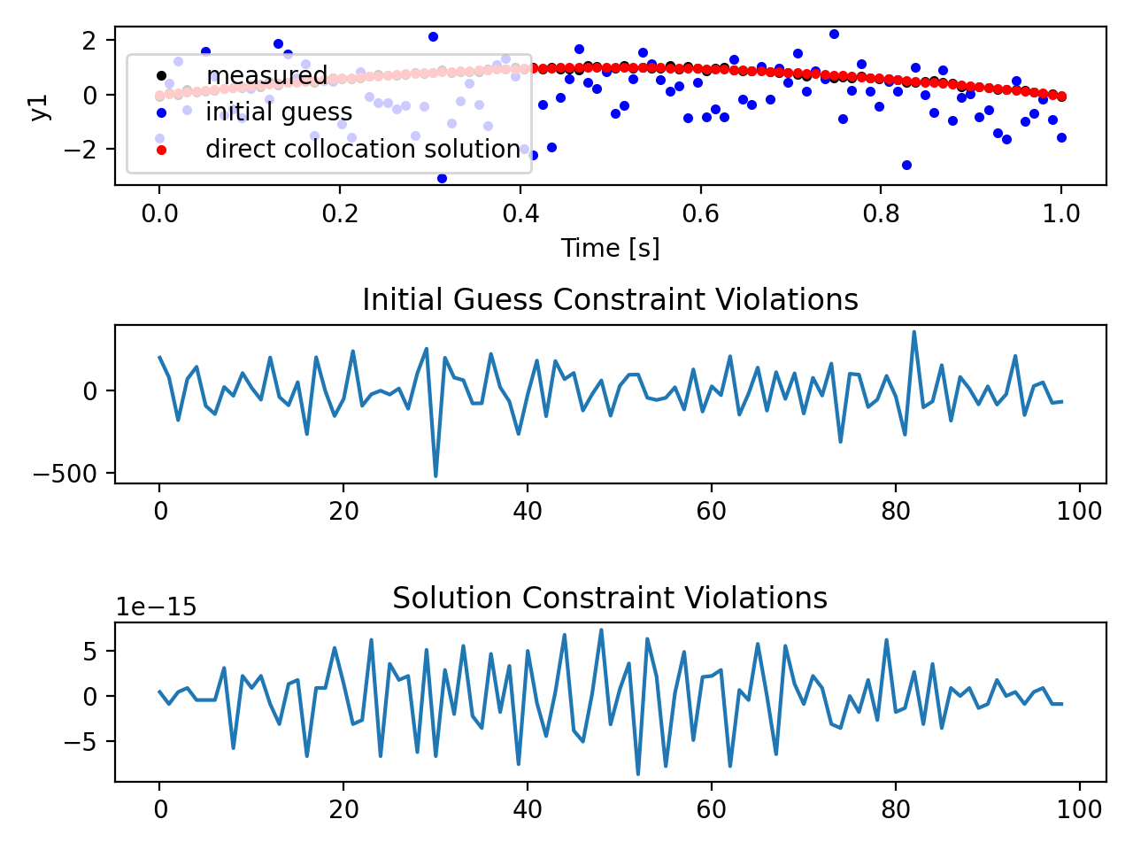
# Plot results
fig_y1, axes_y1 = plt.subplots(3, 1)
legend = ['measured', 'initial guess', 'direct collocation solution']
axes_y1[0].plot(time, y1_m, '.k',
time, initial_guess[:num_nodes], '.b',
time, solution[:num_nodes], '.r')
axes_y1[0].set_xlabel('Time [s]')
axes_y1[0].set_ylabel('y1')
axes_y1[0].legend(legend)
axes_y1[1].set_title('Initial Guess Constraint Violations')
axes_y1[1].plot(prob.con(initial_guess)[:num_nodes - 1])
axes_y1[2].set_title('Solution Constraint Violations')
axes_y1[2].plot(prob.con(solution)[:num_nodes - 1])
plt.tight_layout()
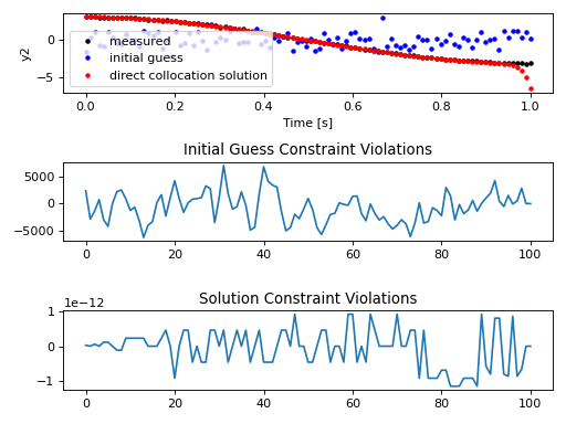
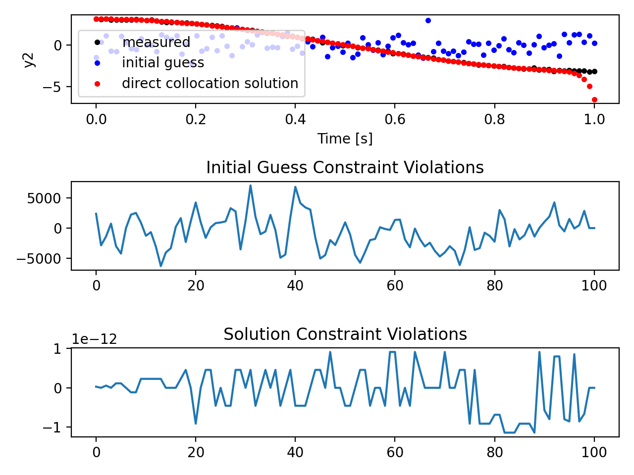
fig_y2, axes_y2 = plt.subplots(3, 1)
axes_y2[0].plot(time, y2_m, '.k',
time, initial_guess[num_nodes:-1], '.b',
time, solution[num_nodes:-1], '.r')
axes_y2[0].set_xlabel('Time [s]')
axes_y2[0].set_ylabel('y2')
axes_y2[0].legend(legend)
axes_y2[1].set_title('Initial Guess Constraint Violations')
axes_y2[1].plot(prob.con(initial_guess)[num_nodes - 1:])
axes_y2[2].set_title('Solution Constraint Violations')
axes_y2[2].plot(prob.con(solution)[num_nodes - 1:])
plt.tight_layout()
plt.show()

Example console output:
******************************************************************************
This program contains Ipopt, a library for large-scale nonlinear optimization.
 Ipopt is released as open source code under the Eclipse Public License (EPL).
         For more information visit http://projects.coin-or.org/Ipopt
******************************************************************************

This is Ipopt version 3.12.8, running with linear solver mumps.
NOTE: Other linear solvers might be more efficient (see Ipopt documentation).

Number of nonzeros in equality constraint Jacobian...:      992
Number of nonzeros in inequality constraint Jacobian.:        0
Number of nonzeros in Lagrangian Hessian.............:        0

Total number of variables............................:      201
                     variables with only lower bounds:        0
                variables with lower and upper bounds:        0
                     variables with only upper bounds:        0
Total number of equality constraints.................:      200
Total number of inequality constraints...............:        0
        inequality constraints with only lower bounds:        0
   inequality constraints with lower and upper bounds:        0
        inequality constraints with only upper bounds:        0

iter    objective    inf_pr   inf_du lg(mu)  ||d||  lg(rg) alpha_du alpha_pr  ls
   0  1.6334109e+00 7.36e+03 8.91e-05   0.0 0.00e+00    -  0.00e+00 0.00e+00   0
   1  1.6283214e+00 1.05e+04 6.49e+02 -11.0 5.34e+00    -  1.00e+00 1.00e+00h  1
   2  2.5566306e-03 2.88e-04 5.62e+00 -11.0 5.62e+00    -  1.00e+00 1.00e+00h  1
   3  2.5551787e-03 1.35e-12 4.99e-05 -11.0 2.07e-02    -  1.00e+00 1.00e+00h  1
   4  2.2437570e-03 9.87e-13 2.99e-11 -11.0 8.90e+00    -  1.00e+00 1.00e+00f  1

Number of Iterations....: 4

                                   (scaled)                 (unscaled)
Objective...............:   2.2437570323119277e-03    2.2437570323119277e-03
Dual infeasibility......:   2.9949274697133673e-11    2.9949274697133673e-11
Constraint violation....:   3.8899404016729276e-14    9.8676622428683913e-13
Complementarity.........:   0.0000000000000000e+00    0.0000000000000000e+00
Overall NLP error.......:   2.9949274697133673e-11    2.9949274697133673e-11


Number of objective function evaluations             = 5
Number of objective gradient evaluations             = 5
Number of equality constraint evaluations            = 5
Number of inequality constraint evaluations          = 0
Number of equality constraint Jacobian evaluations   = 5
Number of inequality constraint Jacobian evaluations = 0
Number of Lagrangian Hessian evaluations             = 0
Total CPU secs in IPOPT (w/o function evaluations)   =      0.024
Total CPU secs in NLP function evaluations           =      0.000

EXIT: Optimal Solution Found.
=========================================
Known value of p = 3.141592653589793
Identified value of p = 3.140935326874292
=========================================
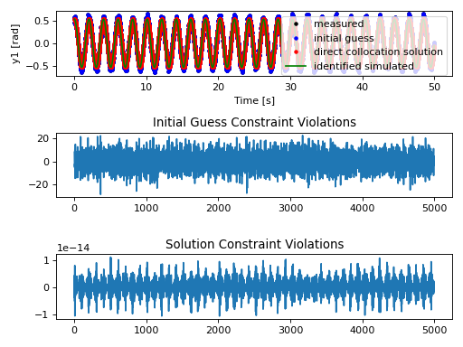
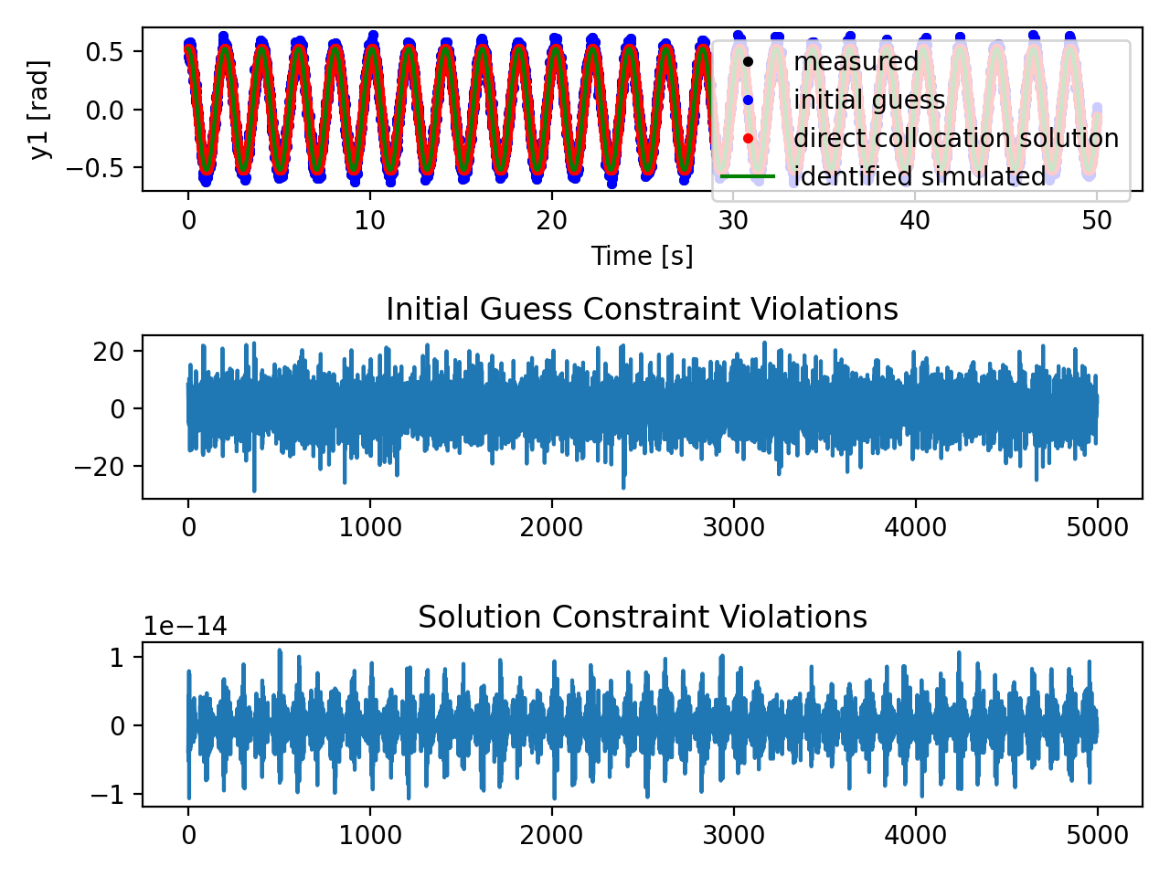
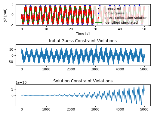
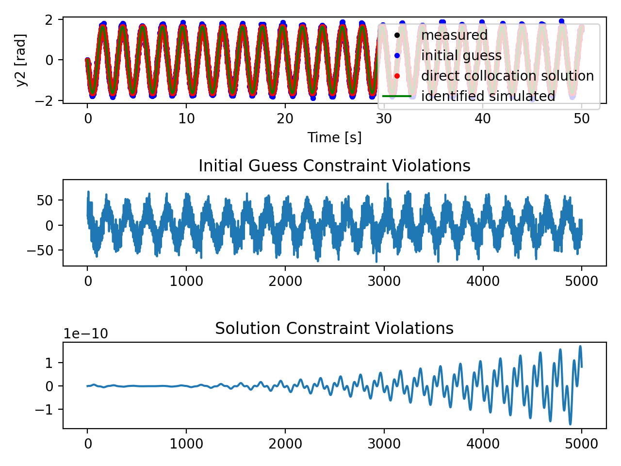
Pendulum Parameter Identification
Identifies a single constant from measured pendulum swing data. The default initial guess for trajectories are the known continuous solution plus artificial Gaussian noise and a random positive value for the parameter.
"""This example is taken from the following paper:

Vyasarayani, Chandrika P., Thomas Uchida, Ashwin Carvalho, and John McPhee.
"Parameter Identification in Dynamic Systems Using the Homotopy Optimization
Approach". Multibody System Dynamics 26, no. 4 (2011): 411-24.

In Section 3.1 there is a simple example of a single pendulum parameter
identification that has many local minima.

For the following differential equations that describe a single pendulum
acting under the influence of gravity, the goals is to identify the
parameter p given noisy measurements of the angle, y1.

               --   --   --            --
               | y1' |   | y2           |
y' = f(y, t) = |     | = |              |
               | y2' |   | -p * sin(y1) |
               --   --   --            --

To run:

    $ python vyasarayani2011.py

Options can be viewed with:

    $ python vyasarayani2011.py -h

"""

import numpy as np
import sympy as sym
from scipy.integrate import odeint
import matplotlib.pyplot as plt
from opty.direct_collocation import Problem
from opty.utils import building_docs


def main(initial_guess, do_plot=False):

    if building_docs():
        do_plot = True

    # Specify the symbolic equations of motion.
    p, t = sym.symbols('p, t')
    y1, y2 = [f(t) for f in sym.symbols('y1, y2', cls=sym.Function)]
    y = sym.Matrix([y1, y2])
    f = sym.Matrix([y2, -p * sym.sin(y1)])
    eom = y.diff(t) - f

    # Generate some data by integrating the equations of motion.
    duration = 50.0
    num_nodes = 5000
    interval = duration / (num_nodes - 1)
    time = np.linspace(0.0, duration, num=num_nodes)

    p_val = 10.0
    y0 = [np.pi / 6.0, 0.0]

    def eval_f(y, t, p):
        return np.array([y[1], -p * np.sin(y[0])])

    y_meas = odeint(eval_f, y0, time, args=(p_val,))
    y1_meas = y_meas[:, 0]
    y2_meas = y_meas[:, 1]

    # Add measurement noise.
    y1_meas += np.random.normal(scale=0.05, size=y1_meas.shape)
    y2_meas += np.random.normal(scale=0.1, size=y2_meas.shape)

    # Setup the optimization problem to minimize the error in the simulated
    # angle and the measured angle.
    def obj(free):
        """Minimize the error in the angle, y1."""
        return interval * np.sum((y1_meas - free[:num_nodes])**2)

    def obj_grad(free):
        grad = np.zeros_like(free)
        grad[:num_nodes] = 2.0 * interval * (free[:num_nodes] - y1_meas)
        return grad

    # The midpoint integration method is preferable to the backward Euler
    # method because no artificial damping is introduced.
    prob = Problem(obj, obj_grad, eom, (y1, y2), num_nodes, interval,
                   integration_method='midpoint')

    num_states = len(y)

    if initial_guess == 'zero':
        print('Using all zeros for the initial guess.')
        # All zeros.
        initial_guess = np.zeros(num_states * num_nodes + 1)
    elif initial_guess == 'randompar':
        print(('Using all zeros for the trajectories initial guess and a '
               'random positive value for the parameter.'))
        # Zeros for the state trajectories and a random positive value for
        # the parameter.
        initial_guess = np.hstack((np.zeros(num_states * num_nodes), 50.0 *
                                   np.random.random(1)))
    elif initial_guess == 'random':
        print('Using random values for the initial guess.')
        # Random values for all unknowns.
        initial_guess = np.hstack((np.random.normal(scale=5.0,
                                                    size=num_states *
                                                    num_nodes), 50.0 *
                                   np.random.random(1)))
    elif initial_guess == 'sysid':
        print(('Using noisy measurements for the trajectory initial guess and '
               'a random positive value for the parameter.'))
        # Give noisy measurements as the initial state guess and a random
        # positive values as the parameter guess.
        initial_guess = np.hstack((y1_meas, y2_meas, 100.0 *
                                   np.random.random(1)))
    elif initial_guess == 'known':
        print('Using the known solution as the initial guess.')
        # Known solution as initial guess.
        initial_guess = np.hstack((y1_meas, y2_meas, 10.0))

    # Find the optimal solution.
    solution, info = prob.solve(initial_guess)
    p_sol = solution[-1]

    # Print the result.
    known_msg = "Known value of p = {}".format(p_val)
    guess_msg = "Initial guess for p = {}".format(initial_guess[-1])
    identified_msg = "Identified value of p = {}".format(p_sol)
    divider = '=' * max(len(known_msg), len(identified_msg))

    print(divider)
    print(known_msg)
    print(guess_msg)
    print(identified_msg)
    print(divider)

    # Simulate with the identified parameter.
    y_sim = odeint(eval_f, y0, time, args=(p_sol,))
    y1_sim = y_sim[:, 0]
    y2_sim = y_sim[:, 1]

    if do_plot:

        # Plot results
        fig_y1, axes_y1 = plt.subplots(3, 1)

        legend = ['measured', 'initial guess',
                  'direct collocation solution', 'identified simulated']

        axes_y1[0].plot(time, y1_meas, '.k',
                        time, initial_guess[:num_nodes], '.b',
                        time, solution[:num_nodes], '.r',
                        time, y1_sim, 'g')
        axes_y1[0].set_xlabel('Time [s]')
        axes_y1[0].set_ylabel('y1 [rad]')
        axes_y1[0].legend(legend)

        axes_y1[1].set_title('Initial Guess Constraint Violations')
        axes_y1[1].plot(prob.con(initial_guess)[:num_nodes - 1])
        axes_y1[2].set_title('Solution Constraint Violations')
        axes_y1[2].plot(prob.con(solution)[:num_nodes - 1])

        plt.tight_layout()

        fig_y2, axes_y2 = plt.subplots(3, 1)

        axes_y2[0].plot(time, y2_meas, '.k',
                        time, initial_guess[num_nodes:-1], '.b',
                        time, solution[num_nodes:-1], '.r',
                        time, y2_sim, 'g')
        axes_y2[0].set_xlabel('Time [s]')
        axes_y2[0].set_ylabel('y2 [rad]')
        axes_y2[0].legend(legend)

        axes_y2[1].set_title('Initial Guess Constraint Violations')
        axes_y2[1].plot(prob.con(initial_guess)[num_nodes - 1:])
        axes_y2[2].set_title('Solution Constraint Violations')
        axes_y2[2].plot(prob.con(solution)[num_nodes - 1:])

        plt.tight_layout()

        plt.show()


if __name__ == "__main__":

    import argparse

    desc = "Run the pendulum parameter identification."
    parser = argparse.ArgumentParser(description=desc)

    msg = "The type of initial guess: sysid, random, known, randompar, zero."
    parser.add_argument('-i', '--initialguess', type=str, help=msg,
                        default='sysid')

    parser.add_argument('-p', '--plot', action="store_true",
                        help="Show result plots.")

    args = parser.parse_args()

    main(args.initialguess, do_plot=args.plot)

Example console output:
Using noisy measurements for the trajectory initial guess and a random positive value for the parameter.

******************************************************************************
This program contains Ipopt, a library for large-scale nonlinear optimization.
 Ipopt is released as open source code under the Eclipse Public License (EPL).
         For more information visit http://projects.coin-or.org/Ipopt
******************************************************************************

This is Ipopt version 3.12.8, running with linear solver mumps.
NOTE: Other linear solvers might be more efficient (see Ipopt documentation).

Number of nonzeros in equality constraint Jacobian...:    49990
Number of nonzeros in inequality constraint Jacobian.:        0
Number of nonzeros in Lagrangian Hessian.............:        0

Total number of variables............................:    10001
                     variables with only lower bounds:        0
                variables with lower and upper bounds:        0
                     variables with only upper bounds:        0
Total number of equality constraints.................:     9998
Total number of inequality constraints...............:        0
        inequality constraints with only lower bounds:        0
   inequality constraints with lower and upper bounds:        0
        inequality constraints with only upper bounds:        0

iter    objective    inf_pr   inf_du lg(mu)  ||d||  lg(rg) alpha_du alpha_pr  ls
   0  0.0000000e+00 8.42e+01 0.00e+00   0.0 0.00e+00    -  0.00e+00 0.00e+00   0
   1  5.0922544e-01 2.04e+01 6.00e+02 -11.0 7.06e+01    -  1.00e+00 1.00e+00h  1
   2  5.9686839e-01 2.79e+00 5.72e+01 -11.0 1.11e+01    -  1.00e+00 1.00e+00h  1
   3  5.7926200e-01 7.31e-02 5.80e+00 -11.0 1.17e+00    -  1.00e+00 1.00e+00h  1
   4  5.7694616e-01 4.40e-04 5.54e-02 -11.0 5.54e-02    -  1.00e+00 1.00e+00h  1
   5  5.0524814e-01 9.16e-02 7.30e-01 -11.0 1.61e+00    -  1.00e+00 5.00e-01f  2
   6  1.3347194e-01 3.11e-02 3.03e-01 -11.0 3.96e-01    -  1.00e+00 1.00e+00h  1
   7  1.3053329e-01 5.72e-04 1.09e-03 -11.0 4.14e-02    -  1.00e+00 1.00e+00h  1
   8  1.3043109e-01 1.40e-05 1.82e-03 -11.0 8.64e-03    -  1.00e+00 1.00e+00h  1
   9  1.2944372e-01 1.88e-05 1.82e-03 -11.0 1.28e-02    -  1.00e+00 1.00e+00h  1
iter    objective    inf_pr   inf_du lg(mu)  ||d||  lg(rg) alpha_du alpha_pr  ls
  10  1.2775048e-01 2.13e-04 1.49e-03 -11.0 3.96e-02    -  1.00e+00 1.00e+00h  1
  11  1.2747061e-01 5.17e-05 5.94e-04 -11.0 1.90e-02    -  1.00e+00 1.00e+00h  1
  12  1.2747075e-01 2.36e-09 1.33e-09 -11.0 8.97e-05    -  1.00e+00 1.00e+00h  1

Number of Iterations....: 12

                                   (scaled)                 (unscaled)
Objective...............:   1.2747074619675813e-01    1.2747074619675813e-01
Dual infeasibility......:   1.3326612572804250e-09    1.3326612572804250e-09
Constraint violation....:   2.3617712230361576e-09    2.3617712230361576e-09
Complementarity.........:   0.0000000000000000e+00    0.0000000000000000e+00
Overall NLP error.......:   2.3617712230361576e-09    2.3617712230361576e-09


Number of objective function evaluations             = 15
Number of objective gradient evaluations             = 13
Number of equality constraint evaluations            = 15
Number of inequality constraint evaluations          = 0
Number of equality constraint Jacobian evaluations   = 13
Number of inequality constraint Jacobian evaluations = 0
Number of Lagrangian Hessian evaluations             = 0
Total CPU secs in IPOPT (w/o function evaluations)   =      3.052
Total CPU secs in NLP function evaluations           =      0.048

EXIT: Optimal Solution Found.
=========================================
Known value of p = 10.0
Initial guess for p = 92.67287860789347
Identified value of p = 10.00138902660221
=========================================